LikelihoodCalc

Let us create a Rate Matrix

row1 <- c(0.0, 1.0, 1.33, 1.0)
row2 <- c(1.0, 0.0, 1.0, 1.33)
row3 <- c(1.33, 1.0, 0.0, 1.0)
row4 <- c(1.0, 1.33, 1.0, 0.0)
rate_mat <- matrix(rbind(c(row1, row2, row3, row4)), nrow = 4)

colnames(rate_mat) <- c("A","C", "G", "T")
rownames(rate_mat) <- c("A","C","G", "T")
rate_mat

##      A    C    G    T
## A 0.00 1.00 1.33 1.00
## C 1.00 0.00 1.00 1.33
## G 1.33 1.00 0.00 1.00
## T 1.00 1.33 1.00 0.00

These are the rates of change. You may see these called exchangeabilities. Now, let’s create a vector of base compositions.

Pi = c(.4, .1, .2, .3)
diagonal_pi <- diag(Pi)

Now we make what is called the Q matrix:

Q_unscaled <- rate_mat * Pi
Q_unscaled

##       A     C     G     T
## A 0.000 0.400 0.532 0.400
## C 0.100 0.000 0.100 0.133
## G 0.266 0.200 0.000 0.200
## T 0.300 0.399 0.300 0.000

Next, we want to scale the Q matrix such that the rows sum to zero.

rowsums <- rowSums(Q_unscaled)
rowsums

##     A     C     G     T 
## 1.332 0.333 0.666 0.999

for (i in 1:4){
  Q_unscaled[i, i] <- -rowsums[1]
}

Q_unscaled

##        A      C      G      T
## A -1.332  0.400  0.532  0.400
## C  0.100 -1.332  0.100  0.133
## G  0.266  0.200 -1.332  0.200
## T  0.300  0.399  0.300 -1.332

Next, we compute a diagonal sum for the matrix. This is used to normalize your Q matrix.

offdiags <- function(mat = matrix){
diag_sum <- sum(diag(mat))
off_diag_sum <- sum(i) - diag_sum
return(off_diag_sum)
}

First we transform by the matrix diagonal of pi.

b <- Q_unscaled * diagonal_pi
b

##         A       C       G       T
## A -0.5328  0.0000  0.0000  0.0000
## C  0.0000 -0.1332  0.0000  0.0000
## G  0.0000  0.0000 -0.2664  0.0000
## T  0.0000  0.0000  0.0000 -0.3996

And this gives us a scaling constant.

scaling <- offdiags(b)

scaledQ <- Q_unscaled/scaling

Now we use this to calculate a likelihood of observing a particular branch length per site:

Pr(Branch Length per site) = scaledQ * BranchLength. For example, if we have our Q matrix, and the branch length is .1, the below are the probabilities of seeing a change between those characters on that branch:

longish_branch <- scaledQ*.05

Now lets imagine we have two taxa, and we have an alignment like so:

Taxon1 = CCAT Taxon2 = CCGT

The probability will look like this:

Likelihood(Data | Model) = Probability(C) * Pr(C --> C) * Pr(C) * Pr(C-->C) * Pr(A) * Pr(A --> G) * Pr(T)* Pr(T-->T)

In code, this will be

Pi[2]*longish_branch[2,2] * Pi[2]*longish_branch[2,2] * Pi[1] * scaledQ[1,3]*Pi[4]*longish_branch[4,4]

## [1] -2.333216e-10

Priors

Priors reflect a prior belief about a variable in the analysis. In this case, for example, we may believe a branch length to be drawn from an exponential distribution. Take a look here at the exponential:

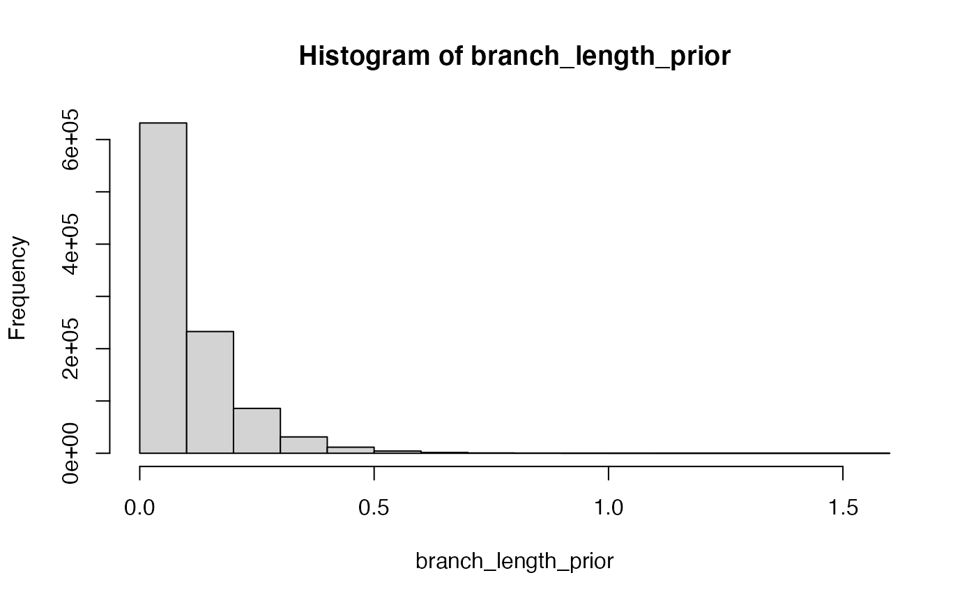
branch_length_prior <- rexp(1000000, 10)
hist(branch_length_prior)

Let’s try the above calculation with a prior included.

branch_length_prior <- rexp(1, 10)

prior_branch <- scaledQ*branch_length_prior
Pi[2]*prior_branch[2,2] * Pi[2]*prior_branch[2,2] * Pi[1] * scaledQ[1,3]*Pi[4]*prior_branch[4,4]

## [1] -6.065097e-12

Homework

Add a couple nucleotides to the alignment. Recalculate the likelihood.

# Work goes here

What happens to your likelihood when you make the branch lengths very long or very short?

# Code here

Reason out why that happens to your likelihood.
In class, we used this loop to generate new branch lengths to connect our two taxa. Figure out how to only view the likelihoods of the invariant characters as you change the branch lengths. What happens to the probability of observing invariant characters as you change the branch lenghts?

for (i in 1:10){
     branch_length <- rexp(1, 10)
     print(branch_length)
     prior_branch <- scaledQ * branch_length
     total_likelihood <- Pi[2]*prior_branch[2, 2] + Pi[2]*prior_branch[2,2] + Pi[1]*prior_branch[1,3] + Pi[4]*prior_branch[4,4]
     print( total_likelihood)
 }

## [1] 0.150883
## [1] -0.01282449
## [1] 0.0725975
## [1] -0.006170515
## [1] 0.003840377
## [1] -0.0003264177
## [1] 0.07182308
## [1] -0.006104693
## [1] 0.08524092
## [1] -0.007245159
## [1] 0.01367261
## [1] -0.00116212
## [1] 0.1820825
## [1] -0.01547633
## [1] 0.2183149
## [1] -0.01855595
## [1] 0.1965378
## [1] -0.01670498
## [1] 0.08382665
## [1] -0.00712495

Parsimony typically measures branch lengths as changes in the data implied by the tree. Likelihood and related methods typically measure them as expected changes per character. A time-scaled tree will express branch legnths in millions of years. What information do you think you need to go from an undated likelihood or parsimony tree to a dated tree?

April Wright

2/22/2022

Let us create a Rate Matrix

Priors

Homework