Molecular Homology Assignment
index.RmdProgressive MSA
Pairwise Multiple Sequence Alignment does exactly what we discussed last week, for all your sequences. Typically, this is performed by first performing a pairwise MSA, as we did above, between the two sequences with the least differences. Then, sequences are added in the order of least differences. Progressive alignments score different alignment possibilities based on the alignment and user-specified scoring matrices, such as BLOSUM 62, or others. Clustal is an example of progressive alignment, but is known to be fairly innaccurate. Below, we use T-COFFEE to get an alignment.
First, we will use T_COFFEE to do alignments. You will find this in the software folder on your RStudio.
We haven’t played with any software yet in this class, so I’ll now have you create a single location for your lab materials. mkdir allows us to make directories. cd allows us to change into the directory.
mkdir lab_one
cd lab_one
Next, you will obtain data:
cp ../data/sh3.fasta .The . above means “here.” It will copy data from a location to where you are.
We’ll now run t_coffee on its default settings (a BLOSUM62 matrix with no gap penalty). First:
/cloud/project/software/t_coffee sh3.fastaNow, we’ll try a gap-opening penalty:
/cloud/project/software/t_coffee sh3.fasta -matrix blosum62mt -gapopen 5 -outfile=gapopen5And one with a gap-extending penalty:
/cloud/project/software/t_coffee sh3.fasta -matrix blosum62mt -gapopen 5 -gapext 5 outfile=gapopen5Try one or two more additional alignments, such as increasing the gap open or extension.
Now, transfer your .aln files to your personal machine.
Use T-Coffee’s online viewer to view them.
As you’re doing this, chat with a partner. What is different between the resulting alignments? Do you have a sense for which you think is “best”?
Iterative Approaches to MSA
Progressive aligners make a set of assumptions, and apply those assumptions to the whole set of sequences across a phylogeny. But many datasets are fairly large, and may have different evolutionary dynamics across the tree. Iterative aligners use tree information to guide the process of making the alignment.
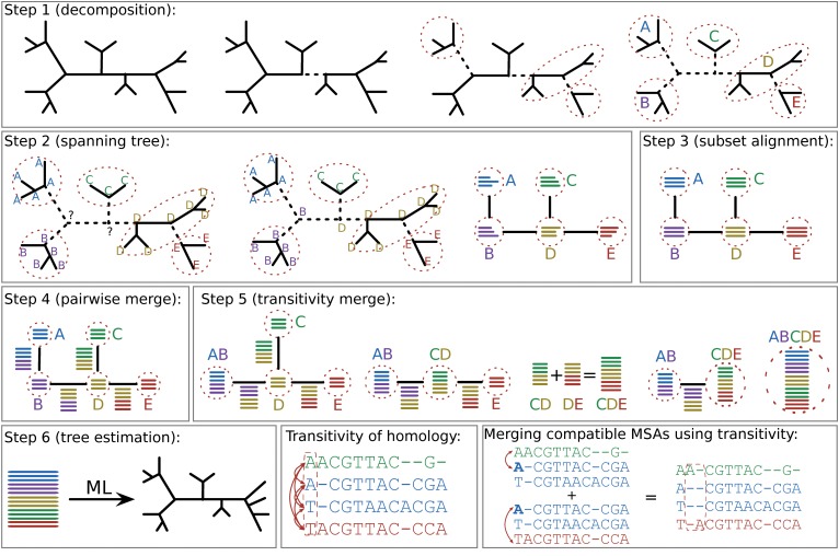
Diagram of Sate/PASTA Algorithm
Now, we will download PASTA:
git clone https://github.com/smirarab/sate-tools-linux.git
git clone https://github.com/smirarab/pasta.git
And we will load a couple libraries required by pasta:
module load java
module load python/3.5.2-anaconda-tensorflow
Now, we build pasta:
python setup.py develop --userChange directories back into your lab_one directory. Copy the data file small.fasta from the data directory to your lab one.
We will use pasta to make an alignment from this small.fasta file.
python ../software/pasta/run_pasta.py -i small.fastaCopy the .aln file and the .tre file to your personal machine. We’re going to look at them quickly.
Choose your own adventure.
Below are two options to improve Pasta’s alignments. Choose one.
Choice of Tree Estimator
Pasta allows us to build a tree for iterative estimation in different ways. FastTree has some known accuracy issues. That’s probably not an issue for an early stage analysis that will be improved. But let’s have a look at what happens if we use a better alignment.
You can change the tree estimator with the option
--tree-estimator raxmlChanging Number of Subsets
Open a tree from one of the iterations in IcyTree. How many clades do you think are on this tree? What size are they? You can edit this with the option
--max-subproblem-size=and choose what you think is the maximum clade size on this tree.
Comparing alignments
As your alignments finish, copy them to your computer - the final alignments will be in the .aln file. We will view our alignment files in Wasabi, which is a simple-browser based alignment.
It can be very hard to appreciate the differences between alignments by eye. We will try making comparisons with FastSP, which gives some at-a-glance comparisons.
Change directories back to your home directory. Clone the FastSP software:
git clone https://github.com/smirarab/FastSP.gitNow, change back to your previous directory with:
cd -You can call FastSP like so:
java -jar /cloud/project/software/FastSP/FastSP.jar -r reference_alignment_file -e estimated_alignment_fileSo, for example, if I wanted to compare the alignment I estimated with Pasta, using FastTree, and the one with Pasta and Raxml, my command would look like
java -jar /cloud/project/software/FastSP/FastSP.jar -r pastajob.marker001.small.aln -e pastajob1.marker001.small.alnFastSP calculates a few summary statistics on alignments. The output should look like:
Reference alignment: /Users/april/Documents/SELUSys2018/lab1/output/pasta_exercise2/smallrax2.marker001.small.aln ...
Estimated alignment: /Users/april/Documents/SELUSys2018/lab1/output/pasta_exercise3/subset_exp.marker001.small.aln ...
MaxLenNoGap= 1027, NumSeq= 32, LenRef= 1169, LenEst= 1180, Cells= 75168
computing ...
Number of shared homologies: 447050
Number of homologies in the reference alignment: 486886
Number of homologies in the estimated alignment: 487792
Number of correctly aligned columns: 716
Number of aligned columns in ref. alignment: 1069
SP-Score 0.9181820795833111
Modeler 0.9164766949847476
SPFN 0.0818179204166889
SPFP 0.0835233050152524
Compression 1.009409751924722
TC 0.6697848456501403
The first line is some information that shouldn’t surprise us too much: the maximum length of sequence in the file without gaps, NumSeq is the number of sequences in the file, the two Lens are the lengths of the alignments (including gaps), and cells are the total number of cells (num seq x number of nucleotides per line, summed for both alignments).
Number of shared homologies refers to how many filled cells are filled in both, or gaps in both. Number of homologies in the reference/estimated alignment is the number of pairs of letters from the input sequences that occur in the same site - this can be larger than the amount of cells, because you’ll make multiple comparisons per column.
Based on these metrics, which alignment do you prefer? What other information would you want to know before choosing an alignment for your project?
Coestimation of MSA and Phylogeny
Phylogenetic esitmation generally assumes that we know the alignment without error. We’ve already seen in our examples cases where we do not get the same alignment between methods. This is particularly true in areas that are hard to align. For example, in the below paper, they estimate a tree for fungi, which are deeply-diverged, and very diverse. The alignment has many problematic regions. What they showed in this paper was that by not accounting for the alignment uncertainty, support was overestimated for their tree hypothesis.
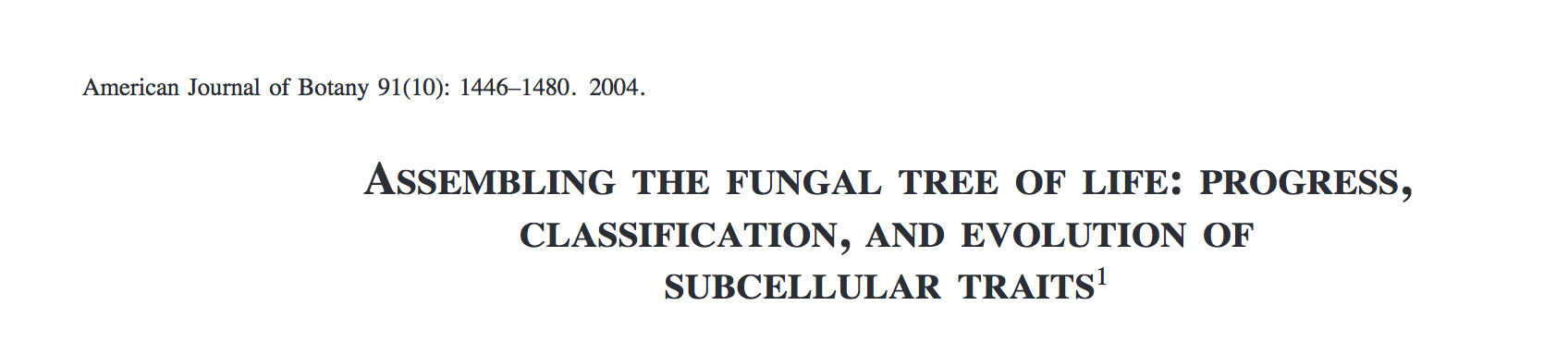
Lutzoni paper
We haven’t talked about Bayesian estimation, so I’m going to say very little on joint estimation of alignment and topology. This is a method that allows for a wide range of models to be deployed in order to estimate both the alignment and the tree, and shows great promise for difficult alignment issues. We have a few floating open labs throughout the semester, so if this is a topic of interest to people, we can revisit it then.
The primary software that performs this analysis is Bali-Phy, which is described here.
Alignment Homework
Some of these questions do not have a right answer.
Feel free to work in groups, and discuss the assignments as needed. However, I do expect you to turn in your own copy, with answers in your own words.
Some algorithms treat a gap as a single penalty value, regardless of how large the gap is. Others assess a gap opening penalty, then a smaller gap extension penalty. When (i.e. what kind of biological scenarios) might you think it might be better to use one algorithm over the other?
Breaking problems into subproblems is a common way to attack a tough problem. In the case of iterative alignments, we break the tree into smaller pieces. In assembling our ddRAD matrices, we build stacks of loci per sample first. Are there biological questions for which you expect this would not be helpful?
References:
- T-Coffee Manual: http://tcoffee.readthedocs.io/en/latest/
- Pasta Algorithm Description: https://www.ncbi.nlm.nih.gov/pmc/articles/PMC4424971/
- Sate Algorithm Description: https://academic.oup.com/sysbio/article/61/1/90/1680002