treesifter Instructor’s Guide

2019-01-10

Introduction

treesiftr is an R package (R Core Team 2018) for visualizing the relationship between phylogenetic trees and phylogenetic data. Phylogenetic trees are crucial to the study of comparative biology, taxonomy, and evolution. However, understanding how to read a phylogenetic tree, and how a phylogenetic tree relates to underlying phylogenetic data, remains challenging.

treesiftr is intended to supplement classroom discussions of phylogeny. Sample slides that could be presented before the activity are included on the software’s GitHub repository. I recommend using treesiftr after a preliminary discussion of tree thinking (such as that found in Baum, Smith, and Donovan (2005)), phylogeny estimation, and how to read phylogenetic trees. After the activity, come back together as a class to talk through the activity and the answers. For more novice classes, it may even be beneficial to do the first five questions, then regroup to discuss the answers before proceding.

How to Use the Instructor’s Guide

treesiftr has two modes. The first is a graphical user interface (GUI). Exercise 01-treesiftr is meant to be used with the graphical interface. The second is the RStudio interface. 02-treesiftr-advanced is meant to be used in RStudio, with executeable code blocks.

The first part of the instructor guide concerns the use of the GUI. The second part explains the RStudio interface, with worked examples.

Tip

Linked text goes to the glossary. If you see a term you don’t recognize, remember you can refresh your memory at the bottom of this worksheet!

01-treesiftr Instructor’s Guide

Learning Objectives

• Be able to count parsimony changes for the displayed characters on the estimated tree.
  • Questions: 1, 2
• Read a phylogenetic tree. Using the information on the tree, apply phylogenetic terminology such as reversal, autapomorphy, and monophyletic to discuss trait and lineage evolution.
  • Questions: 3, 4, 5
• Explain why two characters with the same parsimony score may not have the same likelihood score, and how the number of characters changes the likelihood and parsimony scores.
  • Questions: 6, 7, 8, 9

Navigate to the treesiftr application.

treesiftr works by subsetting a phylogenetic matrix using the start and step arguments. These are found on the left-hand side of the screen. The start argument controls where in the matrix you would like to begin visualizing characters. For example, a start value of 1 would indicate to begin visualizing characters from the first character in the matrix. The step value indicates how many characters at once to visualize. A step value of three would indicate characters should be viewed in threes. For example, if start = 1 and step = 3, the visualization will show characters 1, 2, and 3. The start and end points of character visualizations are noted in the upper left-hand corner of the visualization. For example, in the below, visualization begins with the first character in the dataset. The first three characters (characters 1, 2, and 3) in the data matrix are visualized.

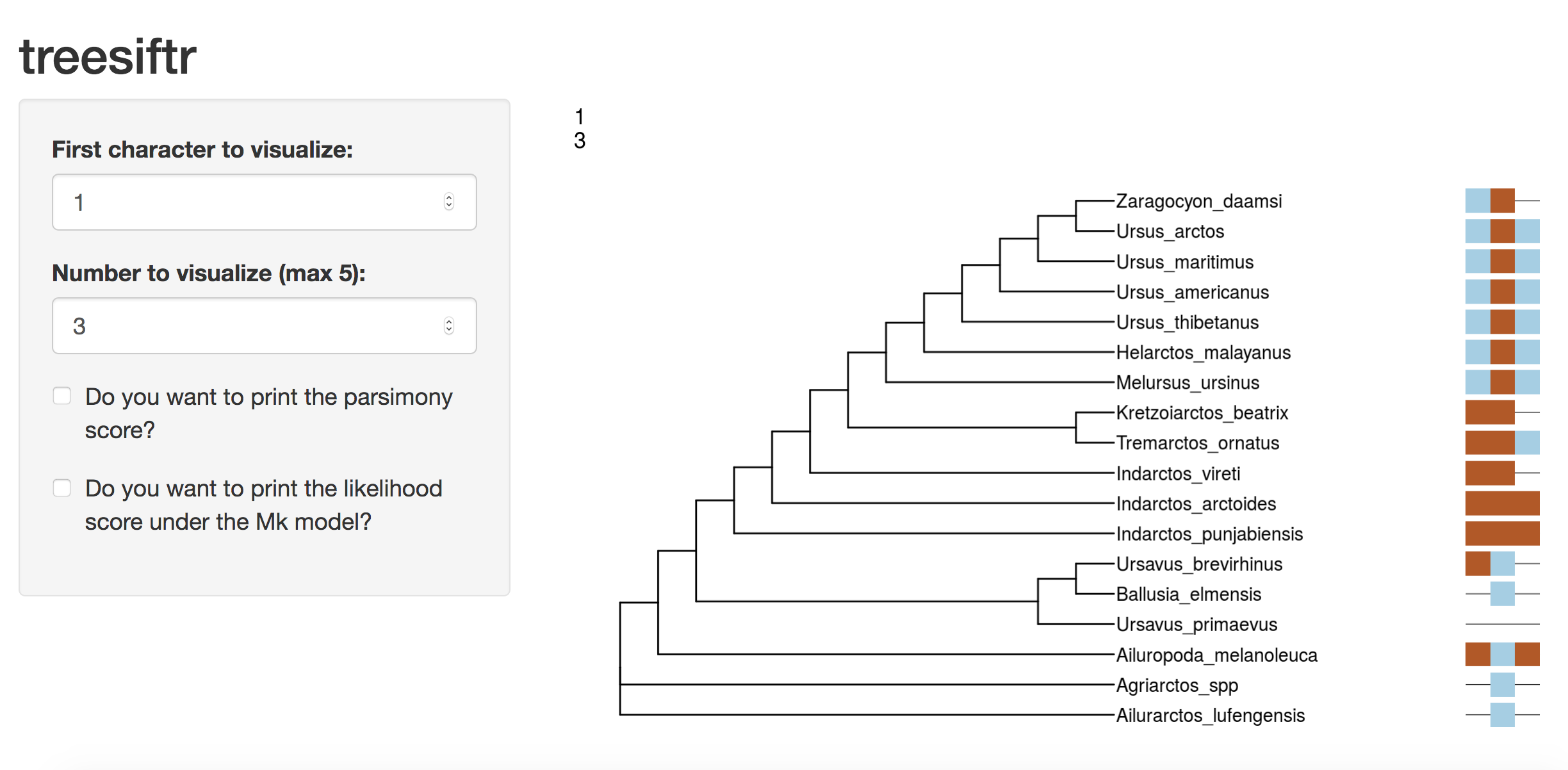
Web Interface example

There are also two checkboxes. The parsimony score checkbox uses Phangorn’s (Schliep 2011, Schliep2017) parsimony scoring algorithm to print the parsimony score of the visualized characters on the tree. The likelihood score is also calculated in Phangorn under the Mk model (Lewis 2001). Leave these unchecked until otherwise noted.

treesiftr works by subsetting a phylogenetic matrix by user input. Then, a parsimony tree is constructed in Phangorn (Schliep 2011, Schliep2017) from the user-defined subset. The tree is scored under both parsimony and Lewis’ Mk model (Lewis 2001) for discrete character data. The data and tree are then visualized using ggtree (Yu et al. 2017), based upon the ggplot2 package (Wickham 2016). This application makes use of Shiny to provide a graphical interface, but there is a second included tutorial for more experienced users of the R statistical language.

Parsimony Questions

1. Visualize characters 1 and 2. What is the parsimony score for this character set? Click “Do you want to print the parsimony score?” in the interface to check your answer.

Instructor’s Note: The answer is two, as viewed in the below screenshot.

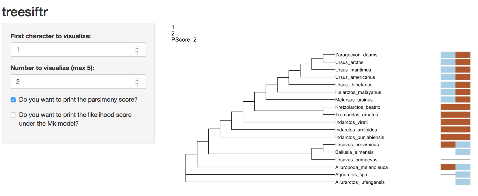
Question One Answer

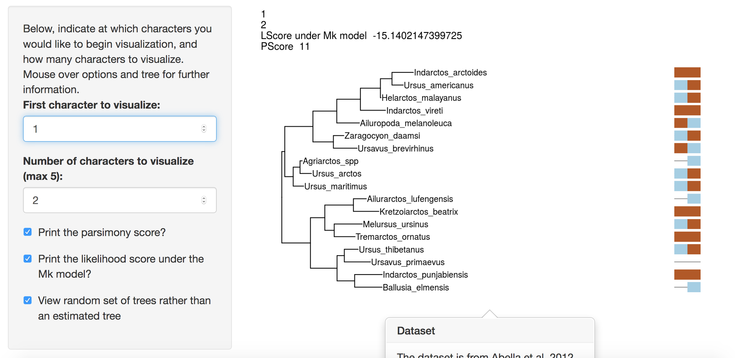
2. Visualize characters 1 and 2. This time, click the “View random set of trees rather than an estimated tree” button in the interface. Are the parsimony scores larger or smaller than those of the character on an estimated tree? Does this make sense to you? Why? Remember to uncheck this box before continuing.

Instructor’s Note: They should be larger. Parsimony estimation will favor the shortest tree while no such criteria is applied to a random tree. Sample output is below, though the exact numbers and distribution will vary.

3. Visualize characters 2 and 3. What monophyletic group from tree 1 is no longer on this tree?

Instructor’s Note: The answer is Ursavus brevirhinus, Ballusia elmensis, and Ursavus primaevus. Ursavus primaevus is no longer sister to Ursavus
brevirhinus and Ballusia elmensis on the tree of character 2-3. Sample output follows.

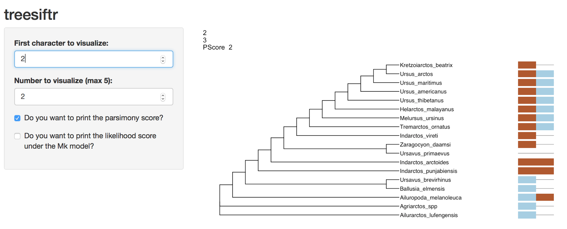
Question Three Answer

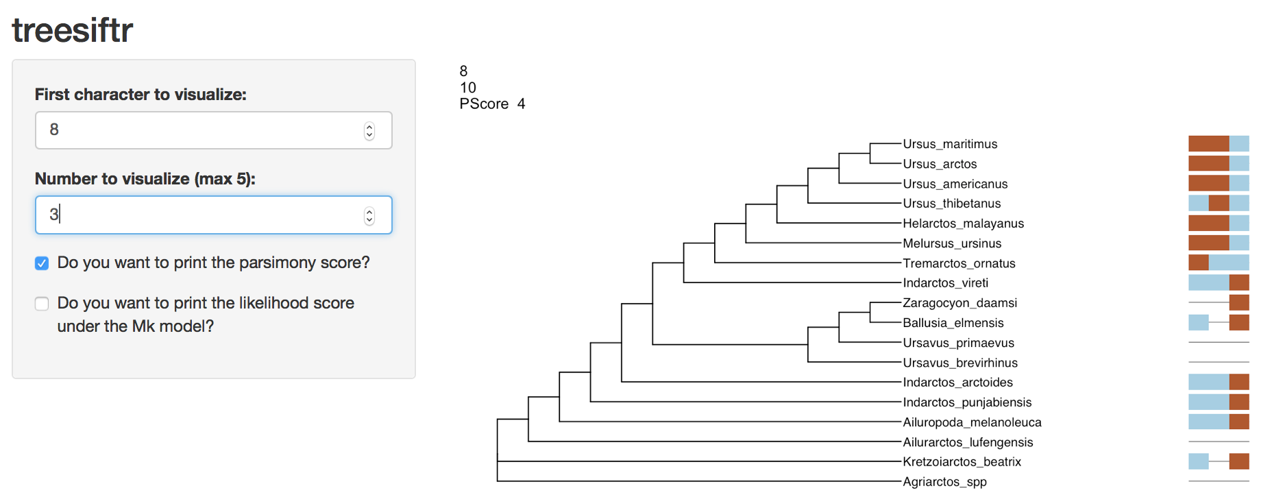
4. Which character, 8, 9 or 10, represents a reversal?

Instructor’s Note: The root of the tree likely blue, with a change to brown on the branch leading to Tremarctos, Melursus, Helarctos, and Ursus. Ursus thibetanus posesses the ancestral blue state, and is the best candidate for reversal.

Question Four Answer

5. What information would we need to decide if the “1” state possesed by Zaragocyon_daamsi in character 52 is an autapomorphy?

Instructor’s Note: To make this decision, we would want to know if there are other bears that are not sampled on this tree that posess this character.

6. Click the switch that says “Do you want to print the likelihood score under the Mk model?” and the switch that says “Do you want to print the parsimony score?”. Does the character set 8, 9, and 10 have the same parsimony score as the character set 9, 10, and 11? How about the same likelihood score?

Instructor’s Notes: It is possible for characters with the same number of parsimony steps to have different likelihood scores.

7. Compare characters 46-49 and 47-50. Why does set 47-50 have a better likelihood than 46-49?

Instructor’s Notes: Answers may vary. But generally, a character (character 46) that implies changes on a fairly short branch is replaced with one implying changes on longer branches.

8. What is the relationship between the likelihood score and increasing the number of characters visualized?

Instructor’s Notes: The likelihood should become more negative (less likely)

9. What is the minimum number adding a parsimony-informative character can add to the parsimony score?

Instructor’s Notes: 1

10. These trees are fully resolved. Based on your exploration of the data, does this degree of resolution make sense?

Instructor’s Notes: For some trees, we can see that there is no character data supporting the grouping. Parsimony software generally displays fully-resolved trees - this may be misleading if little to no data support the grouping!

02-treesiftr-advanced Instructor’s Guide

Instructor’s Note: A sample slide deck for more advanced audiences is included in the folder inst/slides. This slide deck is meant to be viewed in RStudio, as it has executeable code blocks. Hoever, it is also included in HTML format, if this is desireable for presentation. This is simply included as a sample of how one might choose to deliver a lecture to cover some of the phylogenetic terms in this activity. It is not necessary to us this lecture to make use of this activity!

treesiftr works by subsetting a phylogenetic matrix using the start, stop and step arguments. The start argument controls where in the matrix you would like to begin visualizing characters. For example, a start value of 1 would indicate to begin visualizing characters from the first character in the matrix. The stop value indicates what will be the first character in the last visualization. A stop value of 10 would indicate that the first character in the last visualization should be character 10. The step value indicates how many characters at once to visualize. A step value of three would indicate characters should be viewed in threes. For example, if start = 1, stop = 10, and step = 3, 10 visualizations will be produced. The first will visualize characters 1, 2, and 3. The final will be characters 10, 11, and 12.

A maximum parsimony tree is then estimated from each dataset. The tree is scored under both parsimony and Lewis’ Mk model (Lewis 2001) for discrete character data. The data and tree are then visualized using ggtree, based upon the ggplot2 package. This application makes use of Shiny to provide a graphical interface, but in this tutorial, we will use the R Studio interface to visualize our data.

Learning Objectives

• Be able to count parsimony changes for the displayed characters on the estimated tree.
  • Questions: 1, 3
• Apply phylogenetic terminology, such as reversal, autapomorphy, and monophyletic, to discuss trait and lineage evolution.
  • Questions: 2, 4, 5
• Explain why two characters with the same parsimony score may not have the same likelihood score, and how the number of characters changes the likelihood and parsimony scores.
  • Questions: 6, 7, 8, 9
• Use indexing and slicing of data to view desired subsets of data.

Installation

Currently, treesiftr can be installed via the devtools install_github function. treesiftr has a number of required packages. Install and load the below.

Instructor’s Note: This does not auto-execute in the instructor’s guide. phangorn, alignfigr, and ggplot2 are all available via CRAN. ggtree is available via bioconductor. For information on installing bioconductor packages, see here.

#devtools::install_github("wrightaprilm/treesiftr")
library(treesiftr)
library(phangorn)
library(alignfigR)
library(ggtree)
library(ggplot2)

Subsetting the phylogenetic matrix

The first step to making a treesiftr visualization is to select the subset of the phylogenetic matrix that we would like to visualize. This is performed via a function called generate_sliding. The below command will subset the

# Locate package data and read alignment 
fdir <- system.file("extdata", package = "treesiftr") 
aln_path <- file.path(fdir, "bears_fasta.fa")
bears <- read_alignment(aln_path)
# Read in a starting phylogenetic tree
tree <- read.tree(file.path(fdir, "starting_tree.tre"))

# Generate our list of dataframe subsets
sample_df <- generate_sliding(bears, start_char = 1, stop_char = 5, steps = 1)

The result of this is a dataframe, shown below:

sample_df

##   starting_val stop_val step_val
## 1            1        2        1
## 2            2        3        1
## 3            3        4        1
## 4            4        5        1
## 5            5        6        1

This dataframe dispays the start character (the first character that will be visualized) and stop character (the final character that will be visualized).

We can then build trees from each subset:

output_vector <- generate_tree_vis(sample_df = sample_df, alignment =                                                     aln_path, tree = tree, phy_mat = bears)

## Final p-score 2 after  0 nni operations 
## Final p-score 2 after  0 nni operations 
## Final p-score 2 after  0 nni operations 
## Final p-score 2 after  1 nni operations 
## Final p-score 2 after  1 nni operations

The above code saves the trees to a vector, but does not visualize them. They can be viauslized by naming the vector, like so:

output_vector 

## [[1]]
## NULL
## 
## [[2]]
## NULL
## 
## [[3]]
## NULL
## 
## [[4]]
## NULL
## 
## [[5]]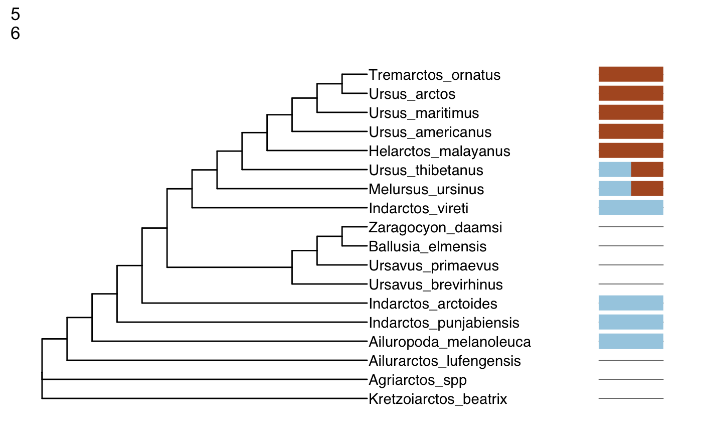

Phangorn (Schliep 2011, Schliep2017) requires a starting tree to estimate a parsimony tree. We specify the tree we read in earlier for this purpose. The trees, which were generated with ggtree (Yu et al. 2017) have been saved to a vector, which can be displayed in its entirety, or subsetted to look at specific trees.

Questions

1. Visualize characters 1 and 2. What is the parsimony score for this character set? Once you have answered this question,check your answer by adding the parismony score using the pscore argument:

output_vector <- generate_tree_vis(sample_df = sample_df, alignment =                                                     aln_path, tree = tree, phy_mat = bears,
                                   pscore = TRUE)

## Final p-score 2 after  0 nni operations 
## Final p-score 2 after  0 nni operations 
## Final p-score 2 after  0 nni operations 
## Final p-score 2 after  1 nni operations 
## Final p-score 2 after  1 nni operations

output_vector

## [[1]]
## NULL
## 
## [[2]]
## NULL
## 
## [[3]]
## NULL
## 
## [[4]]
## NULL
## 
## [[5]]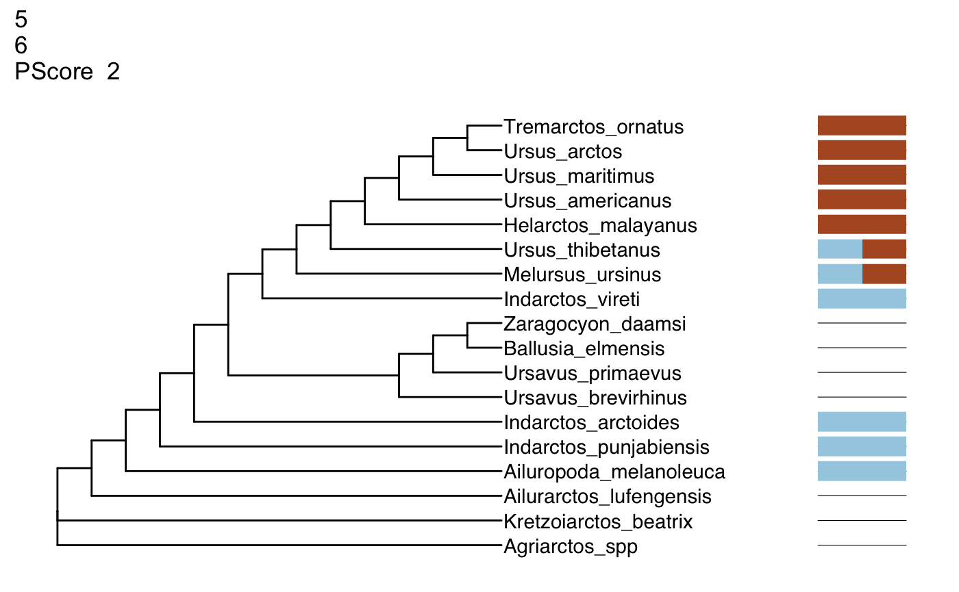

Instructor’s Note: The answer is two, as viewed in the first visualization in the vector.

2. Visualize characters 1 and 2. This time, click the “View random set of trees rather than an estimated tree” button in the interface. Are the parsimony scores larger or smaller than those of the character on an estimated tree? Does this make sense to you? Why?

Instructor’s Note: They should be larger. Parsimony estimation will favor the shortest tree while no such criteria is applied to a random tree. This can be checked like so:

sample_df <- generate_sliding(bears, start_char = 31, stop_char = 32, steps = 3)

output_vector <- generate_tree_vis(sample_df = sample_df, alignment =                                                     aln_path, tree = tree, phy_mat = bears,
                      pscore = TRUE, random_tree = TRUE)

## [1] 20
## [1] 18

output_vector[1]

## [[1]]
## NULL

3. Visualize character set 2-3 and 3-4. What monophyletic group from the tree for characters 2-3 is no longer on the tree for characters 3-4?

Instructor’s Note: The answer is Ursavus brevirhinus and Ballusia elmensis. This clade is broken up on the tree for characters 3-4, in which Ballusia elmensis is sister to Zaragocyon_daamsi.

4. View a tree of characters 8 - 10. Which character, 8, 9 or 10, represents a reversal from a derived state to ancestral?

Instructor’s Note: The root of the tree likely blue, with a change to brown on the branch leading to Tremarctos, Melursus, Helarctos, and Ursus. Ursus thibetanus posesses the ancestral blue state, and is the best candidate for reversal. This can be verified like so:

sample_df <- generate_sliding(bears, start_char = 8, stop_char = 9, steps = 2)

output_vector <- generate_tree_vis(sample_df = sample_df, alignment =                                                     aln_path, tree = tree, phy_mat = bears,
                                   pscore = TRUE)

## Final p-score 4 after  0 nni operations 
## Final p-score 4 after  1 nni operations

output_vector[1]

## [[1]]
## NULL

5. What information would we need to decide if the “1” state possesed by Zaragocyon_daamsi in character 52 is an autapomorphy?

Instructor’s Note: To make this decision, we would want to know if there are other bears that are not sampled on this tree that posess this character. We can view the tree like so:

sample_df <- generate_sliding(bears, start_char = 52, stop_char = 53, steps = 1)

output_vector <- generate_tree_vis(sample_df = sample_df, alignment =                                                     aln_path, tree = tree, phy_mat = bears,
                                   pscore = TRUE)

## Final p-score 2 after  0 nni operations 
## Final p-score 2 after  0 nni operations

output_vector[1]

## [[1]]
## NULL

6. Do all characters with the same parsimony score have the same likelihood score? You can add the likelihood score to the visualization using the below code:

output_vector <- generate_tree_vis(sample_df = sample_df, alignment =                                                     aln_path, tree = tree, phy_mat = bears, 
                                   pscore = TRUE, lscore = TRUE)

## Final p-score 2 after  0 nni operations 
## Final p-score 2 after  0 nni operations

output_vector

## [[1]]
## NULL
## 
## [[2]]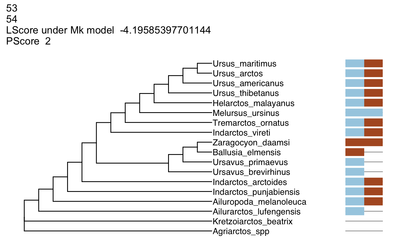

Instructor’s Notes: It is possible for characters with the same number of parsimony steps to have different likelihood scores.

7. Compare characters 46-49 and 47-50. Why does set 47-50 have a better likelihood than 46-49?

Instructor’s Notes: Answers may vary. But generally, a character (character 46) that implies changes on a fairly short branch is replaced with one implying changes on longer branches.

sample_df <- generate_sliding(bears, start_char = 46, stop_char = 49, steps = 3)

output_vector <- generate_tree_vis(sample_df = sample_df, alignment =                                                     aln_path, tree = tree, phy_mat = bears, 
                                   pscore = TRUE, lscore = TRUE)

## Final p-score 7 after  0 nni operations 
## Final p-score 7 after  0 nni operations 
## Final p-score 5 after  1 nni operations 
## Final p-score 5 after  1 nni operations

output_vector

## [[1]]
## NULL
## 
## [[2]]
## NULL
## 
## [[3]]
## NULL
## 
## [[4]]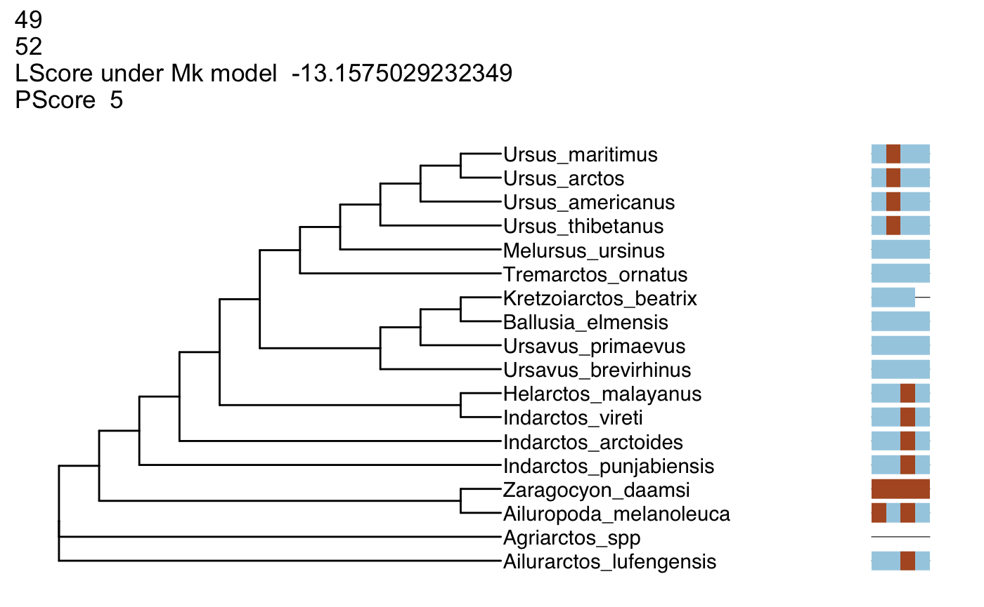

8. What is the relationship between the likelihood score and increasing the number of characters visualized? > Instructor’s Notes: The likelihood should become more negative (less likely)

9. What is the minimum number adding a parsimony-informative character can add to the parsimony score?

Instructor’s Notes: 1

10. These trees are fully resolved. Based on your exploration of the data, does this degree of resolution make sense? Take a look at characters 1-3, for example. Does displaying a fully resolved tree make sense for these characters?

Instructor’s Notes: For some trees, we can see that there is no character data supporting the grouping. Parsimony software generally displays fully-resolved trees - this may be misleading if little to no data support the grouping! In our case, we’re seeing strong influence of the starting tree.

Glossary

Ancestral State: A character state possessed by the ancestor of a group

Autapomorphy: A character state that is unique to a specific taxon.

Derived State: A character state that is different from the ancestral state.

Likelihood Score: The likelihood of the observed data under a specific model.

Maximum likelihood: A phylogenetic optimatlity criterion under which phylogenetic data are modeled according to sets of assumptions. Under this criterion, the tree that has the best (“maximum”) likelihood score under the assumed model is to be preferred.

Maximum parsimony: A phylogenetic optimality criterion. This criterion holds that the tree implying the fewest changes in the characters used to generate it should be preferred.

Monophyletic: A group on a phylogeny of an ancestor and all of its descendents.

Parsimony Score: The number of changes implied by a character on a tree.

Resolved: A node that is bifucating, leaving two descendent lineages.

Reversal: A change from the derived state back to the ancestral state.

References

Baum, David A., Stacey DeWitt Smith, and Samuel S. S. Donovan. 2005. “The Tree-Thinking Challenge.” Science 310 (5750). American Association for the Advancement of Science: 979–80. https://doi.org/10.1126/science.1117727.

Lewis, Paul O. 2001. “A Likelihood Approach to Estimating Phylogeny from Discrete Morphological Character Data.” Systematic Biology 50 (6). Oxford University Press: 913–25. https://doi.org/10.1080/106351501753462876.

R Core Team. 2018. R: A Language and Environment for Statistical Computing. Vienna, Austria: R Foundation for Statistical Computing. https://www.R-project.org/.

Schliep, K.P. 2011. “Phangorn: Phylogenetic Analysis in R.” Bioinformatics 27 (4): 592–93. https://doi.org/10.1093/bioinformatics/btq706.

Wickham, Hadley. 2016. Ggplot2: Elegant Graphics for Data Analysis. Springer-Verlag New York. http://ggplot2.org.

Yu, Guangchuang, David Smith, Huachen Zhu, Yi Guan, and Tommy Tsan-Yuk Lam. 2017. “Ggtree: An R Package for Visualization and Annotation of Phylogenetic Trees with Their Covariates and Other Associated Data.” Methods in Ecology and Evolution 8 (1): 28–36. https://doi.org/10.1111/2041-210X.12628.