RevBayes Total Evidence Tree Estimation
RB_Total_Evidence_Tutorial.RmdOverview
This tutorial demonstrates how to specify the models used in a Bayesian “total-evidence” phylogenetic analysis of extant and fossil species, combining morphological and molecular data as well as stratigraphic range data from the fossil record (e.g., Ronquist et al. 2012; Zhang et al. 2016; Gavryushkina et al. 2016). We begin with a concise introduction to the models used in this analysis in section Introduction, followed by a detailed example analysis in section Exercise demonstrating how to apply these models in RevBayes(Höhna, Landis, and Heath 2017) and use Markov chain Monte Carlo (MCMC) to estimate the posterior distribution of dated phylogenies for data collected from living and fossil bears (family Ursidae).
Requirements
Required Software
This tutorial requires that you download and install the latest release of RevBayes(Höhna, Landis, and Heath 2017), which is available for Mac OS X, Windows, and Linux operating systems. Directions for downloading and installing the software are available on the program webpage: http://revbayes.com. The exercise provided also requires additional programs for editing text files and visualizing output. The following are very useful tools for working with RevBayes:
A good text editor – if you do not already have one that you like, we recommend one that has features for syntax coloring, easy navigation between different files, line numbers, etc. Good options include Sublime Text or Atom, which are available for Mac OSX, Windows, and Linux.
Tracer – for visualizing and assessing numerical parameter samples from
RevBayesIcyTree – a web-hosted phylogenetic tree visualization tool that is supported for Firefox or Google Chrome browsers
FigTree – a tree visualization program
Introduction
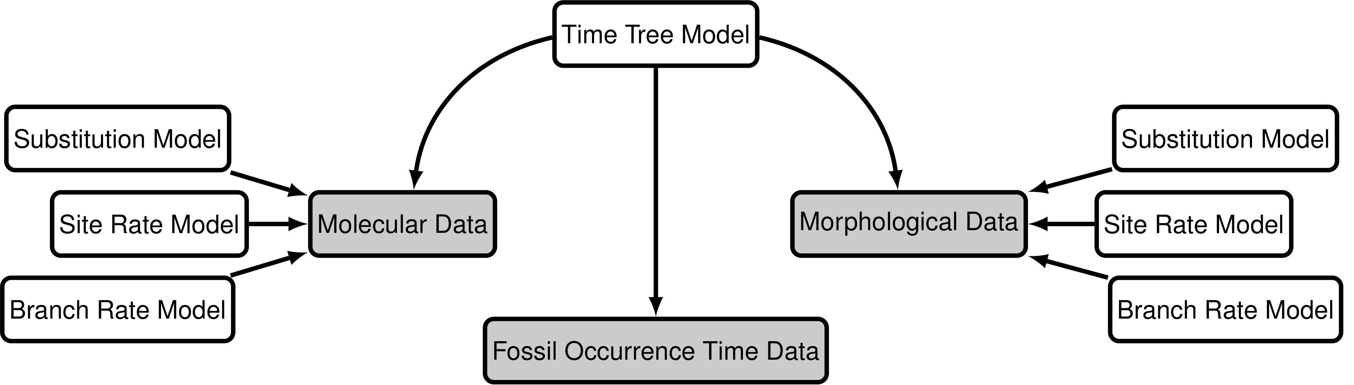
The “total-evidence” analysis described in this tutorial uses a probabilistic graphical model (Höhna et al. 2014) integrating three separate likelihood components or data partitions (Fig. 1): one for molecular data one for morphological data, and one for fossil stratigraphic range data. In addition, all likelihood components are conditioned on a tree topology with divergence times, which is modeled according to a separate prior component.
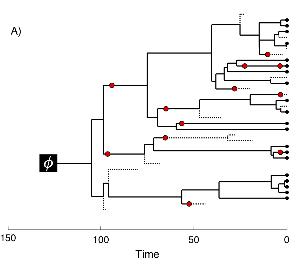
In figure 2 we provide an example of the type of tree estimated from a total-evidence analysis. This example shows the complete tree (Fig. 2A) and the sampled or reconstructed tree (Fig. 2B). Importantly, we are interested in estimating the topology, divergence times, and fossil sample times of the reconstructed tree (Fig. 2B). We will describe the distinction between these two trees in the section Intro to FBD.
| Complete Tree | Sampled Tree |
|---|---|
 |
 |
Lineage Diversification and Sampling
The joint prior distribution on tree topologies and divergence times of living and extinct species used in this tutorial is described by the fossilized birth-death (FBD) process (Stadler 2010; Heath, Huelsenbeck, and Stadler 2014). This model simply treats the fossil observations as part of the process governing the tree topology and branch times (the node in Fig. 3). The fossilized birth-death process provides a model for the distribution of speciation times, tree topology, and lineage samples before the present (e.g.,non-contemporaneous samples like fossils or viruses). This type of tree is shown in figure 2. Importantly, this model can be used with or without character data for the historical samples. Thus, it provides a reasonable prior distribution for analyses combining morphological or DNA data for both extant and fossil taxa—i.e.,the so-called “total-evidence” approaches described by Ronquist et al. (2012) and extended by Zhang et al. (2016) and Gavryushkina et al. (2016). When matrices of discrete morphological characters for both living and fossil species are unavailable, the fossilized birth-death model imposes a time structure on the tree by marginalizing over all possible attachment points for the fossils on the extant tree (Heath, Huelsenbeck, and Stadler 2014), therefore, some prior knowledge of phylogenetic relationships is important.
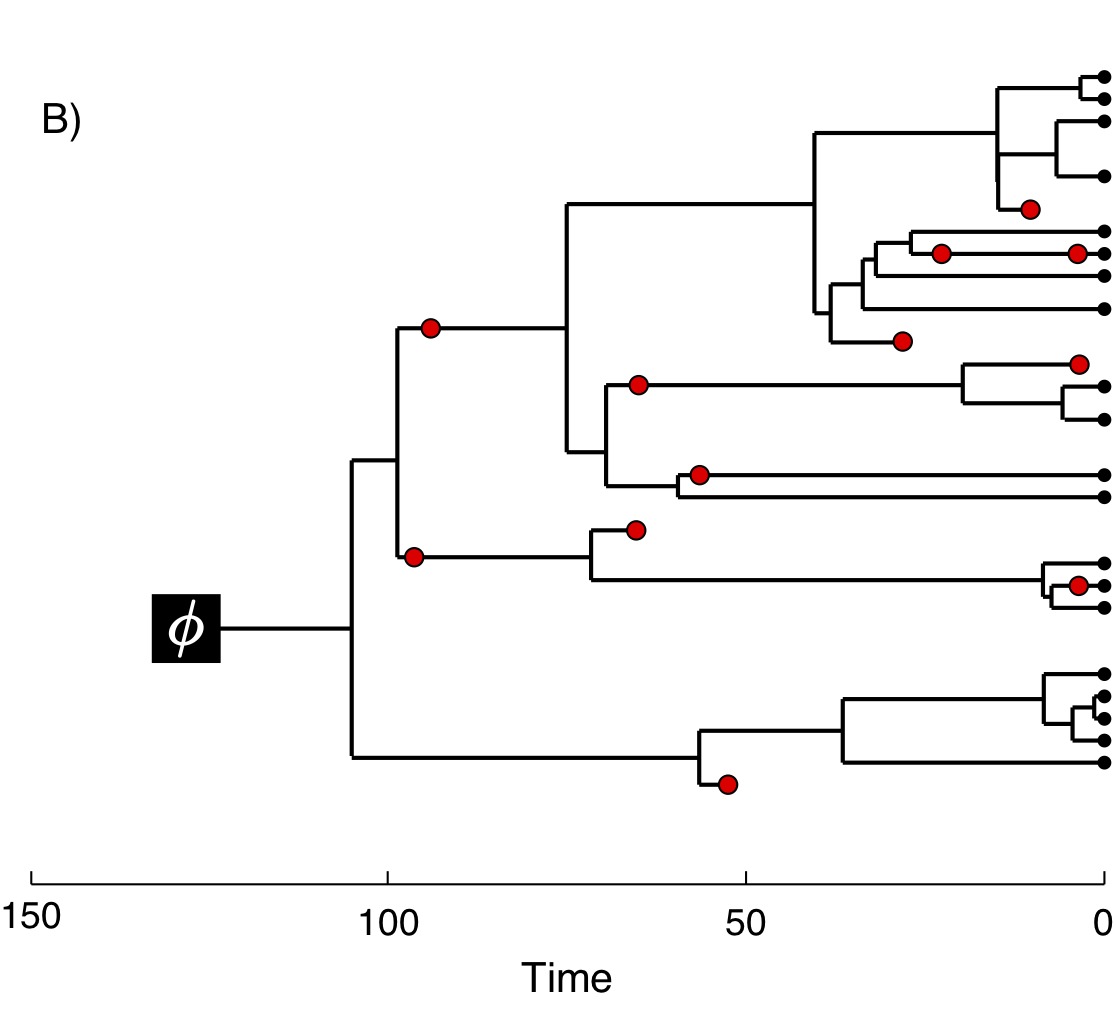
The FBD model (Fig. 3) describes the probability of the tree and fossils conditional on the birth-death parameters: \(f[\mathcal{T} \mid \lambda, \mu, \rho, \psi, \phi]\), where \(\mathcal{T}\) denotes the tree topology, divergence times, fossil occurrence times, and the times at which the fossils attach to the tree. The birth-death parameters \(\lambda\) and \(\mu\) denote the speciation and extinction rates, respectively. The “fossilization rate” or “fossil recovery rate” is denoted \(\psi\) and describes the rate at which fossils are sampled along lineages of the complete tree. The sampling probability parameter \(\rho\) represents the probability that an extant species is sampled, and \(\phi\) represents the time at which the process originated.
In the example FBD tree shown in figure 2, the diversification process originates at time \(\phi\), giving rise to \(n=20\) species in the present, with both sampled fossils (red circles) and extant species (black circles). All of the lineages represented in figure 2A (both solid and dotted lines) show the complete tree. This is the tree of all extant and extinct lineages generated by the process. The complete tree is distinct from the reconstructed tree (Fig. 2B) which is the tree representing only the lineages sampled as extant taxa or fossils. Fossil observations (red circles in figure 2) are recovered over the lifetime of the process along the lineages of the complete tree. If a lineage does not have any descendants sampled in the present, it is lost and cannot be observed, these are the dotted lines in figure 2A. The probability must be conditioned on the origin time of the process \(\phi\). The origin (\(\phi\)) of a birth-death process is the starting time of the stem lineage, thus this conditions on a single lineage giving rise to the tree.
An important characteristic of the FBD model is that it accounts for the probability of sampled ancestor-descendant pairs (Foote 1996). Given that fossils are sampled from lineages in the diversification process, the probability of sampling fossils that are ancestors to taxa sampled at a later date is correlated with the turnover rate (\(r=\mu/\lambda\)) and the fossil recovery rate (\(\psi\)). This feature is important, particularly for datasets with many sampled fossils. In the example (Fig. 2), several of the fossils have sampled descendants. These fossils have solid black lines leading to the present.
Incorporating Fossil Occurrence Time Uncertainty
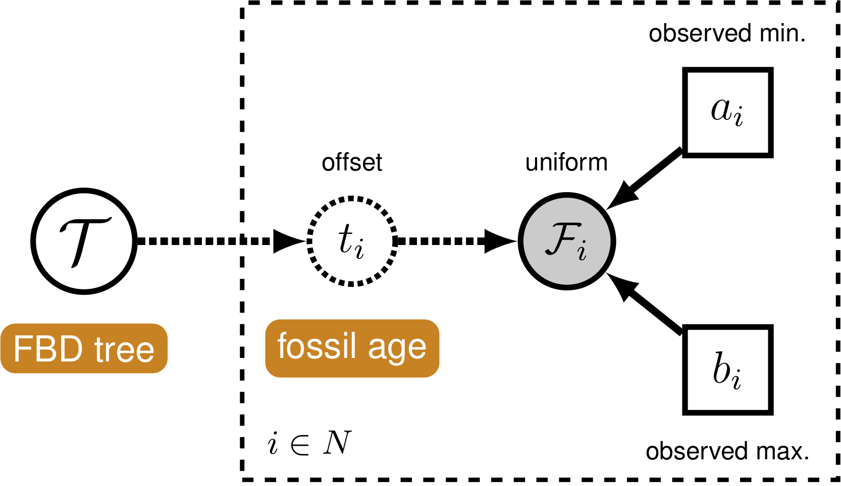
In order to account for uncertainty in the ages of our fossil species, we can incorporate intervals on the ages of our represented fossil species. These intervals can be stratigraphic ranges or measurement standard error. We do this by assuming each fossil can occur with uniform probability anywhere within its observed interval. This is somewhat different from the typical approach to node calibration. Here, instead of treating the calibration density as an additional prior distribution on the tree, we treat it as the likelihood of our fossil data given the tree parameter. Specifically, we assume the likelihood of a particular fossil observation \(\mathcal{F}_i\) is equal to one if the fossil’s inferred age on the tree \(t_i\) falls within its observed time interval \((a_i,b_i)\), and zero otherwise: \[f[\mathcal{F}_i \mid a_i, b_i, t_i] = \begin{cases}
1 & \text{if } a_i < t_i < b_i\\
0 & \text{otherwise}
\end{cases}\] In other words, we assume the likelihood is equal to one if the inferred age is consistent with the data observed. We can represent this likelihood in RevBayesusing a distribution that is proportional to the likelihood, i.e.,non-zero when the likelihood is equal to one (Fig. 4). This model component represents the observed in the modular graphical model shown in figure 1.
It is worth noting that this is not technically the appropriate way to model fossil data that are actually observed as stratigraphic ranges. In paleontology, a stratigraphic range represents the interval of time between the first and last appearences of a fossilized species. Thus, this range typically represents multiple fossil specimens observed at different times along a single lineage. An extension of the fossilized birth-death process that is a distribution on stratigraphic ranges has been described by Stadler et al. (2017). This model is not yet fully implemented in RevBayes.
Nucleotide Sequence Evolution
The model component for the molecular data uses a general time-reversible model of nucleotide evolution and gamma-distributed rate heterogeneity across sites (the and in Fig. 1). This model of sequence evolution is covered thoroughly in the Substitution Models tutorial.
Lineage-Specific Rates of Sequence Evolution
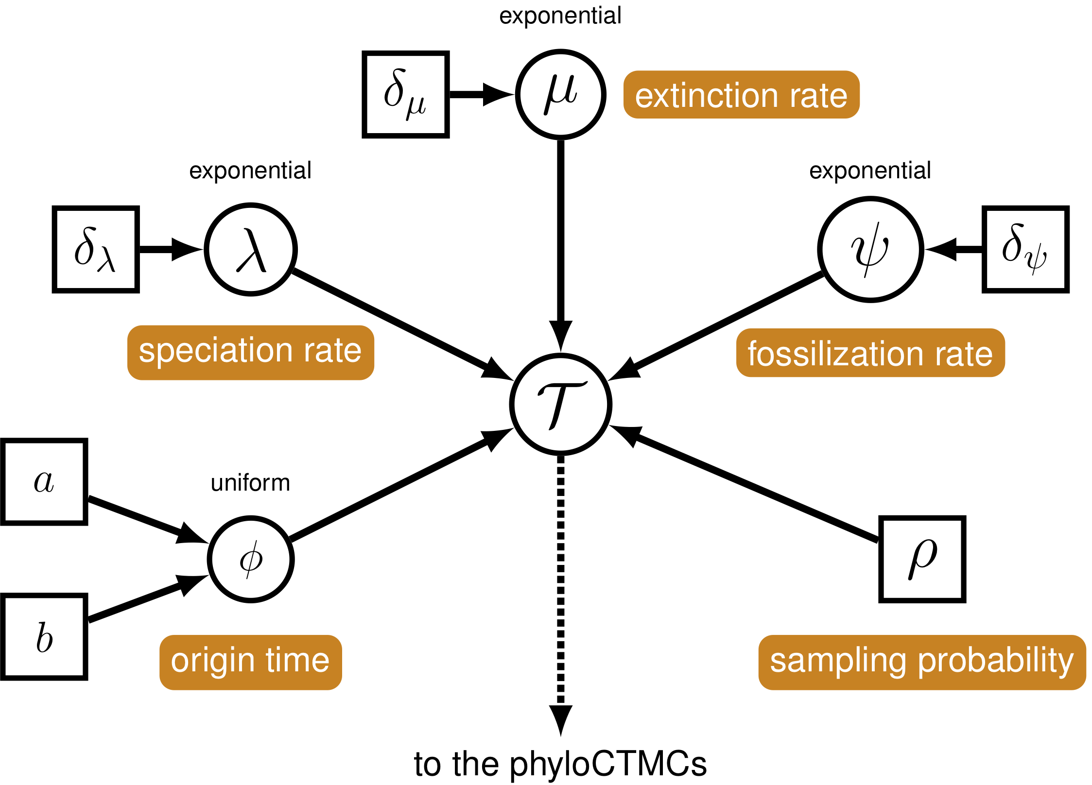
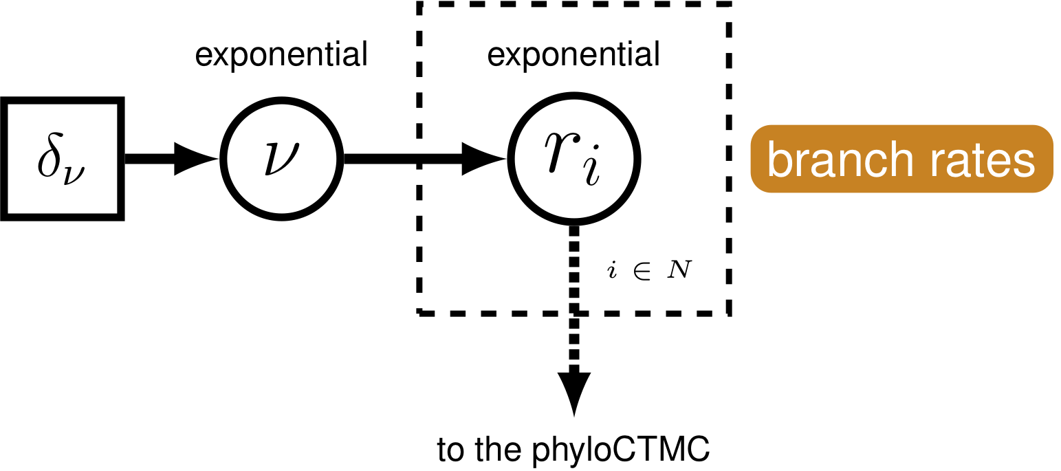
Rates of nucleotide sequence evolution can vary widely among lineages, and so models that account for this variation by relaxing the assumption of a strict molecular clock (Zuckerkandl and Pauling 1962) can allow for more accurate estimates of substitution rates and divergence times (Drummond et al. 2006). The simplest type of relaxed clock model assumes that lineage-specific substitution rates are independent or “uncorrelated”. One example of such an uncorrelated relaxed model is the uncorrelated exponential relaxed clock, in which the substitution rate for each lineage is assumed to be independent and identically distributed according to an exponential density (Fig. 5). This is the for the (i.e.,Fig. 1) that we will use in this tutorial. Another possible uncorrelated relaxed clock model is the uncorrelated lognormal model, described in the Relaxed Clocks tutorial (also see Thorne and Kishino 2002; T. A. Heath and Moore 2014).
Morphological Character Evolution
For the vast majority of extinct species, fossil morphology is the primary source of phylogenetically informative characters. Therefore, an appropriate model of morphological character evolution is needed to reliably infer the positions of these species in a phylogenetic analysis. The Mk model (Lewis 2001) uses a generalized Jukes-Cantor matrix to allow for the incorporation of morphology into likelihood and Bayesian analyses. In its simplest form, this model assumes that characters change states symmetrically—that a given character is as likely to transition from a one state to another as it is to reverse. In this tutorial we will consider only binary morphological characters, i.e.,characters that are observed in one of two states, 0 or 1. For example, the assumption of the single-rate Mk model applied to our binary character would mean that a change from a 0 state to a 1 state is as likely as a change from a 1 state to a 0 state. This assumption is equivalent to assuming that the stationary probability of being in a 1 state is equal to \(1/2\).
In this tutorial, we will apply a single-rate Mk model as a prior on binary morphological character change. If you are interested extensions of the Mk model that relax the assumptions of symmetric state change, please see Discrete Morphology tutorial.
Because of the way morphological data are collected, we need to exercise caution in how we model the data. Traditionally, phylogenetic trees were built from morphological data using parsimony. Therefore, only parsimony informative characters were collected—that is, characters that are useful for discriminating between phylogenetic hypotheses under the maximum parsimony criterion. This means that many morphological datasets do not contain invariant characters or autapomorphies, as these are not parsimony informative. However, by excluding these slow-evolving characters, estimates of the branch lengths can be inflated (Felsenstein 1992; Lewis 2001). Therefore, it is important to use models that can condition on this data-acquisition bias. RevBayeshas two ways of doing this: one is used for datasets in which only parsimony informative characters are observed; the other is for datasets in which parsimony informative characters and parsimony uninformative variable characters (such as autapomorphies) are observed.
The Morphological Clock
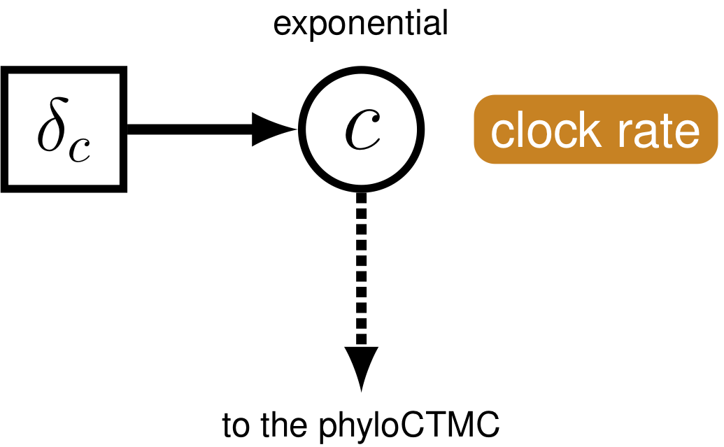
Just like with the molecular data (section Intro to GTR and UExp), our observations of discrete morphological characters are conditional on the rate of change along each branch in the tree. This model component defines the of the in the generalized graphical model shown in figure 1. The relaxed clock model we described for the molecular data in section Intro to GTR and UExp it allows the substitution rate to vary through time and among lineages. For the morphological data, we will instead use a “strict clock” model (Zuckerkandl and Pauling 1962), in which the rate of discrete character change is assumed to be constant throughout the tree. The strict clock is the simplest morphological branch rate model we can construct (graphical model shown in Fig. 6.
Example: Estimating the Phylogeny and Divergence Times of Fossil and Extant Bears
In this exercise, we will combine different types of data from 22 species of extant and extinct bears to estimate a posterior distribution of calibrated time trees for this group. We have molecular sequence data for ten species, which represent all of the eight living bears and two extinct species sequenced from sub-fossil specimens (Arctodus simus, Ursus spelaeus). The sequence alignment provided is a 1,000 bp fragment of the cytochrome-b mitochondrial gene (Krause et al. 2008). The morphological character matrix unites 18 taxa (both fossil and extant) with 62 binary (states 0 or 1) characters (Abella et al. 2012). For the fossil species, occurrence times are obtained from the literature or fossil databases like the Fossilworks PaleoDB or the Fossil Calibration Database, or from your own paleontological expertise. The 14 fossil species used in this analysis are listed in Table 1 along with the age range for the species and relevant citation. Finally, there are two fossil species (Parictis montanus, Ursus abstrusus) for which we do not have morphological character data (or molecular data) and we must use prior information about their phylogenetic relationships to incorporate these taxa in our analysis. This information will be applied using clade constraints.
| Taxon | Age | Citation |
|---|---|---|
| Parictis montanus | 33.9–37.2 | (Clark and Guensburg 1972; Krause et al. 2008) |
| Zaragocyon daamsi | 20–22.8 | (Ginsburg and Morales 1995; Abella et al. 2012) |
| Ballusia elmensis | 13.7–16 | (Ginsburg and Morales 1998; Abella et al. 2012) |
| Ursavus primaevus | 13.65–15.97 | (Andrews and Tobien 1977; Abella et al. 2012) |
| Ursavus brevihinus | 15.97–16.9 | (Heizmann, Ginsburg, and Bulot 1980; Abella et al. 2012) |
| Indarctos vireti | 7.75–8.7 | (Montoya, Alcalá, and Morales 2001; Abella et al. 2012) |
| Indarctos arctoides | 8.7–9.7 | (Geraads et al. 2005; Abella et al. 2012) |
| Indarctos punjabiensis | 4.9–9.7 | (Baryshnikov 2002; Abella et al. 2012) |
| Ailurarctos lufengensis | 5.8–8.2 | (Jin et al. 2007; Abella et al. 2012) |
| Agriarctos spp. | 4.9–7.75 | (Abella, Montoya, and Morales 2011; Abella et al. 2012) |
| Kretzoiarctos beatrix | 11.2–11.8 | (Abella, Montoya, and Morales 2011; Abella et al. 2012) |
| Arctodus simus | 0.012–2.588 | (Churcher, Morgan, and Carter 1993; Krause et al. 2008) |
| Ursus abstrusus | 1.8–5.3 | (Bjork 1970; Krause et al. 2008) |
| Ursus spelaeus | 0.027–0.25 | (Loreille et al. 2001; Krause et al. 2008) |
Tutorial Format
This tutorial follows a specific format for issuing instructions and information.
The boxed instructions guide you to complete tasks that are not part of the RevBayessyntax, but rather direct you to create directories or files or similar.
Information describing the commands and instructions will be written in paragraph-form before or after they are issued.
All command-line text, including all Revsyntax, are given in monotype font. Furthermore, blocks of Revcode that are needed to build the model, specify the analysis, or execute the run are given in separate shaded boxes. For example, we will instruct you to create a constant node called rho that is equal to 1.0 using the <- operator like this:
rho <- 1.0It is important to be aware that some PDF viewers may render some characters given as differently. Thus, if you copy and paste text from this PDF, you may introduce some incorrect characters. Because of this, we recommend that you type the instructions in this tutorial or copy them from the scripts provided.
Data and Files
This part of the workshop will take place in RevBayes.
In my course’s vignettes directory, find RB_Total_Evidence. Change directories into it.
In the data folder, you will find the following files:
bears_taxa.tsv: a tab-separated table listing every bear species (both fossil and extant) and their occurrence dates. For extant taxa, the occurrence date is0.0(i.e.,the present) and for fossil species, the occurrence date is equal to the mean of the age range (the ranges are defined in a separate file).bears_cytb.nex: an alignment in NEXUS format of 1,000 bp of cytochrome b sequences for 10 bear species. This alignment includes 8 living bears and 2 extinct sub-fossil bears.bears_morphology.nex: a matrix of 62 discrete, binary (coded0or1) morphological characters for 18 species of fossil and extant bears.bears_fossil_intervals.tsv: a tab-separated table containing the age ranges (minimum and maximum in millions of years) for 14 fossil bears.
Getting Started
Create a new directory (in RB_TotalEvidenceDating_FBD_Tutorial) called . (If you do not have this folder, please refer to the directions in section Data files)
When you execute RevBayesin this exercise, you will do so within the main directory, RB_TotalEvidenceDating_FBD_Tutorial, thus, if you are using a Unix-based operating system, we recommend that you add the RevBayesbinary to your path.
Creating RevFiles
For complex models and analyses, it is best to create Revscript files that will contain all of the model parameters, moves, and functions. In this exercise, you will work primarily in your text editor[^1] and create a set of modular files that will be easily managed and interchanged. You will write the following files from scratch and save them in the scripts directory:
mcmc_TEFBD.Rev: the masterRevfile that loads the data, the separate model files, and specifies the monitors and MCMC sampler.model_FBDP_TEFBD.Rev: specifies the model parameters and moves required for the fossilized birth-death prior on the tree topology, divergence times, fossil occurrence times, and diversification dynamics.model_UExp_TEFBD.Rev: specifies the components of the uncorrelated exponential model of lineage-specific substitution rate variation.model_GTRG_TEFBD.Rev: specifies the parameters and moves for the general time-reversible model of sequence evolution with gamma-distributed rates across sites (GTR+\(\Gamma\)).model_Morph_TEFBD.Rev: specifies the model describing discrete morphological character change (binary characters) under a strict morphological clock.
All of the files that you will create are also provided in the RevBayestutorial repository[^2]. Please refer to these files to verify or troubleshoot your own scripts.
Start the Master RevFile and Import Data
Open your text editor and create the master Revfile called in the scripts directory.
Enter the Revcode provided in this section in the new model file.
The file you will begin in this section will be the one you load into RevBayeswhen you’ve completed all of the components of the analysis. In this section you will begin the file and write the Revcommands for loading in the taxon list and managing the data matrices. Then, starting in section Model FBD, you will move on to writing module files for each of the model components. Once the model files are complete, you will return to editing mcmc_TEFBD.Rev and complete the Revscript with the instructions given in section Complete MCMC].
Load Taxon List
Begin the Revscript by loading in the list of taxon names from the bears_taxa.tsv file using the readTaxonData() function.
taxa <- readTaxonData("data/bears_taxa.tsv")This function reads a tab-delimited file and creates a variable called taxa that is a list of all of the taxon names relevant to this analysis. This list includes all of the fossil and extant bear species names in the first columns and a single age value in the second column. The ages provided are either 0.0 for extant species or the average of the age range for fossil species (see the table of ages above).
Load Data Matrices
RevBayesuses the function readDiscreteCharacterData() to load a data matrix to the workspace from a formatted file. This function can be used for both molecular sequences and discrete morphological characters.
Load the cytochrome-b sequences from file and assign the data matrix to a variable called cytb.
cytb <- readDiscreteCharacterData("data/bears_cytb.nex") Next, import the morphological character matrix and assign it to the variable morpho.
morpho <- readDiscreteCharacterData("data/bears_morphology.nex")Add Missing Taxa
In the descriptions of the files in section Data Files, we mentioned that the two data matrices have different numbers of taxa. Thus, we must add any taxa that are not found in the molecular (cytb) partition (i.e.,are only found in the fossil data) to that data matrix as missing data (with ? in place of all characters), and do the same with the morphological data partition (morpho). In order for all the taxa to appear on the same tree, they all need to be part of the same dataset, as opposed to present in separate datasets. This ensures that there is a unified taxon set that contains all of our tips.
cytb.addMissingTaxa( taxa )
morpho.addMissingTaxa( taxa )
Create Helper Variables
Before we begin writing the Revscripts for each of the model components, we need to instantiate a couple “helper variables” that will be used by downstream parts of our model specification files. These variables will be used in more than one of the module files so it’s best to initialize them in the master file.
Create a new constant node called n_taxa that is equal to the number of species in our analysis (22).
n_taxa <- taxa.size() Next, create a workspace variable called mvi. This variable is an iterator that will build a vector containing all of the MCMC moves used to propose new states for every stochastic node in the model graph. Each time a new move is added to the vector, mvi will be incremented by a value of 1.
mvi = 1One important distinction here is that mvi is part of the RevBayesworkspace and not the hierarchical model. Thus, we use the workspace assignment operator = instead of the constant node assignment <-.
Save your current working version of mcmc_TEFBD.Rev in the scripts directory.
We will now move on to the next Revfile and will complete mcmc_TEFBD.Rev in section Complete MCMC.
The Fossilized Birth-Death Process
Open your text editor and create the fossilized birth-death model file called in the scripts directory.
Enter the Revcode provided in this section in the new model file.
This file will define the models described in sections Intro to FBD and Intro to TipSampling above. If necessary, please review the graphical models depicted for the fossilized birth-death process (Fig. 3) and the likelihood of the tip sampling process (Fig. 3).
Speciation and Extinction Rates
Two key parameters of the FBD process are the speciation rate (the rate at which lineages are added to the tree, denoted by \(\lambda\) in Fig. 3) and the extinction rate (the rate at which lineages are removed from the tree, \(\mu\) in Fig. 3). We’ll place exponential priors on both of these values. Each parameter is assumed to be drawn independently from a different exponential distribution with rates \(\delta_{\lambda}\) and \(\delta_{\mu}\) respectively (see Fig. 3). Here, we will assume that \(\delta_{\lambda} = \delta_{\mu} = 10\). Note that an exponential distribution with \(\delta = 10\) has an expected value (mean) of \(1/10\).
Create the exponentially distributed stochastic nodes for the speciation_rate and extinction_rate using the ~ operator.
speciation_rate ~ dnExponential(10)
extinction_rate ~ dnExponential(10)
For every stochastic node we declare, we must also specify proposal algorithms (called moves) to sample the value of the parameter in proportion to its posterior probability. If a move is not specified for a stochastic node, then it will not be estimated, but fixed to its initial value.
The rate parameters for extinction and speciation are both positive, real numbers (i.e.,non-negative floating point variables). For both of these nodes, we will use a scaling move (mvScale()), which proposes multiplicative changes to a parameter. Many moves also require us to set a tuning value, called lambda for mvScale(), which determine the size of the proposed change. Here, we will use three scale moves for each parameter with different values of lambda. By using multiple moves for a single parameter, we will improve the mixing of the Markov chain.
moves[mvi++] = mvScale(speciation_rate, lambda=0.01, weight=1)
moves[mvi++] = mvScale(speciation_rate, lambda=0.1,  weight=1)
moves[mvi++] = mvScale(speciation_rate, lambda=1.0,  weight=1)

moves[mvi++] = mvScale(extinction_rate, lambda=0.01, weight=1)
moves[mvi++] = mvScale(extinction_rate, lambda=0.1,  weight=1)
moves[mvi++] = mvScale(extinction_rate, lambda=1,    weight=1)
You will also notice that each move has a specified weight. This option allows you to indicate how many times you would like a given move to be performed at each MCMC cycle. The way that we will run our MCMC for this tutorial will be to execute a schedule of moves at each step in our chain instead of just one move per step, as is done in MrBayes (Ronquist and Huelsenbeck 2003) or BEAST (Drummond et al. 2012; Bouckaert et al. 2014). Here, if we were to run our MCMC with our current vector of 6 moves, then our move schedule would perform 6 moves at each cycle. Within a cycle, an individual move is chosen from the move list in proportion to its weight. Therefore, with all six moves assigned weight=1, each has an equal probability of being executed and will be performed on average one time per MCMC cycle. For more information on moves and how they are performed in RevBayes, please refer to the Introduction to MCMC and Substitution Models tutorials.
In addition to the speciation (\(\lambda\)) and extinction (\(\mu\)) rates, we may also be interested in inferring diversification (\(\lambda - \mu\)) and turnover (\(\mu/\lambda\)). Since these parameters can be expressed as a deterministic transformation of the speciation and extinction rates, we can monitor (that is, track the values of these parameters, and print them to a file) their values by creating two deterministic nodes using the := operator.
diversification := speciation_rate - extinction_rate
turnover := extinction_rate/speciation_rate
Probability of Sampling Extant Taxa
All extant bears are represented in this dataset. Therefore, we will fix the probability of sampling an extant lineage (\(\rho\) in Fig. 3) to 1. The parameter rho will be specified as a constant node using the <- operator.
rho <- 1.0Because \(\rho\) is a constant node, we do not have to assign a move to this parameter.
The Fossil Sampling Rate
Since our data set includes serially sampled lineages, we must also account for the rate of sampling back in time. This is the fossil sampling (or recovery) rate (\(\psi\) in Fig. 3), which we will instantiate as a stochastic node (named psi). As with the speciation and extinction rates (Sect. FBD-Speciation & Extinction]), we will use an exponential prior on this parameter and use scale moves to sample values from the posterior distribution.
psi ~ dnExponential(10)
moves[mvi++] = mvScale(psi, lambda=0.01, weight=1)
moves[mvi++] = mvScale(psi, lambda=0.1,  weight=1)
moves[mvi++] = mvScale(psi, lambda=1,    weight=1)
The Origin Time
We will condition the FBD process on the origin time (\(\phi\) in Fig. 3) of bears, and we will specify a uniform distribution on the origin age. For this parameter, we will use a sliding window move (mvSlide). A sliding window samples a parameter uniformly within an interval (defined by the half-width delta). Sliding window moves can be tricky for small values, as the window may overlap zero. However, for parameters such as the origin age, there is little risk of this being an issue.
origin_time ~ dnUnif(37.0, 55.0)
moves[mvi++] = mvSlide(origin_time, delta=0.01, weight=5.0)
moves[mvi++] = mvSlide(origin_time, delta=0.1,  weight=5.0)
moves[mvi++] = mvSlide(origin_time, delta=1,    weight=5.0)
Note that we specified a higher move weight for each of the proposals operating on origin_time than we did for the three previous stochastic nodes. This means that our move schedule will propose five times as many updates to origin_time than it will to speciation_rate, extinction_rate, or psi.
The FBD Distribution Object
All the parameters of the FBD process have now been specified. The next step is to use these parameters to define the FBD tree prior distribution, which we will call fbd_dist.
fbd_dist = dnFBDP(origin=origin_time, lambda=speciation_rate, mu=extinction_rate, psi=psi, rho=rho, taxa=taxa)Clade Constraints
Note that we created the distribution as a workspace variable using the workspace assignment operator =. This is because we still need to include a topology constraint in our final specification of the tree prior. Specifically, we do not have any morphological or molecular data for the fossil species Ursus abstrusus. Therefore, in order to use the age of this fossil as an observation, we need to specify to which clade it belongs. In this case, Ursus abstrusus belongs to the subfamily Ursinae, so we define a clade for the total group Ursinae including Ursus abstrusus.
clade_ursinae = clade("Melursus_ursinus", "Ursus_arctos", "Ursus_maritimus",
                      "Helarctos_malayanus", "Ursus_americanus", "Ursus_thibetanus",
                      "Ursus_abstrusus", "Ursus_spelaeus")
Then we can specify the final constrained tree prior distribution by creating a vector of constraints, and providing it along with the workspace FBD distribution to the constrained topology distribution. Here we use the stochastic assignment operator ~ to create a stochastic node for our constrained, FBD-tree variable (called fbd_tree).
constraints = v(clade_ursinae)
fbd_tree ~ dnConstrainedTopology(fbd_dist, constraints=constraints)
It is important to recognize that we do not know if Ursus abstrusus is a crown or stem Ursinae. Because of this, we defined this clade constraint so that it constrained the total group Ursinae and this uncertainty is taken into account. As a result, our MCMC will marginalize over both stem and crown positions of U. abstrusus and sample the phylogeny in proportion to its posterior probability, conditional on our model and data.
Additionally, we do not have morphological data for the fossil species Parictis montanus. However, we will not create a clade constraint for this taxon because it is a very old, stem-fossil bear. Thus, the MCMC may propose to place this taxon anywhere in the tree (except within the clade constraint we made above). This allows us to account for the maximum amount of uncertainty in the placement of P. montanus.
Moves on the Tree Topology and Node Ages
Next, in order to sample from the posterior distribution of trees, we need to specify moves that propose changes to the topology (mvFNPR) and node times (mvNodeTimeSlideUniform). Included with these moves is a proposal that will collapse or expand a fossil branch (mvCollapseExpandFossilBranch). This will change a fossil that is a sampled ancestor (see Fig. 2 and Sect. Intro to FBD) so that it is on its own branch and vice versa. In addition, when conditioning on the origin time, we also need to explicitly sample the root age (mvRootTimeSlideUniform).
moves[mvi++] = mvFNPR(fbd_tree, weight=15.0)
moves[mvi++] = mvCollapseExpandFossilBranch(fbd_tree, origin_time, weight=6.0)
moves[mvi++] = mvNodeTimeSlideUniform(fbd_tree, weight=40.0)
moves[mvi++] = mvRootTimeSlideUniform(fbd_tree, origin_time, weight=5.0)
Sampling Fossil Occurrence Ages
Next, we need to account for uncertainty in the age estimates of our fossils using the observed minimum and maximum stratigraphic ages provided in the file bears_fossil_intervals.tsv. First, we read this file into a matrix called intervals.
intervals = readDataDelimitedFile(file="data/bears_fossil_intervals.tsv", header=true)Next, we loop over this matrix. For each fossil observation, we create a uniform random variable representing the likelihood. Remember, we can represent the fossil likelihood using any uniform distribution that is non-zero when the likelihood is equal to one (Sect. Tip Sampling).
For example, if \(t_i\) is the inferred fossil age and \((a_i,b_i)\) is the observed stratigraphic interval, we know the likelihood is equal to one when \(a_i < t_i < b_i\), or equivalently \(t_i - b_i < 0 < t_i - a_i\). So let’s represent the likelihood using a uniform random variable uniformly distributed in \((t_i - b_i, t_i - a_i)\) and clamped at zero.
for(i in 1:intervals.size())
{
    taxon  = intervals[i][1]
    a_i = intervals[i][2]
    b_i = intervals[i][3]

    t[i] := tmrca(fbd_tree, clade(taxon))

    fossil[i] ~ dnUniform(t[i] - b_i, t[i] - a_i)
    fossil[i].clamp( 0 )
}
Finally, we add a move that samples the ages of the fossil nodes on the tree.
moves[mvi++] = mvFossilTimeSlideUniform(fbd_tree, origin_time, weight=5.0)Monitoring Parameters of Interest using Deterministic Nodes
There are additional parameters that may be of particular interest to us that are not directly inferred as part of this graphical model. As with the diversification and turnover nodes specified in section FBD-Speciation & Extinction, we can create deterministic nodes to sample the posterior distributions of these parameters. Create a deterministic node called num_samp_anc that will compute the number of sampled ancestors in our fbd_tree.
num_samp_anc := fbd_tree.numSampledAncestors()We are also interested in the age of the most-recent-common ancestor (MRCA) of all living bears. To monitor the age of this node in our MCMC sample, we must use the clade() function to identify the node. Importantly, since we did not include this clade in our constraints that defined fbd_tree, this clade will not be constrained to be monophyletic. Once this clade is defined, we can instantiate a deterministic node called age_extant with the tmrca() function that will record the age of the MRCA of all living bears.
clade_extant = clade("Ailuropoda_melanoleuca","Tremarctos_ornatus","Melursus_ursinus",
                    "Ursus_arctos","Ursus_maritimus","Helarctos_malayanus",
                    "Ursus_americanus","Ursus_thibetanus")
age_extant := tmrca(fbd_tree, clade_extant)
In the same way we monitored the MRCA of the extant bears, we can also monitor the age of a fossil taxon that we may be interested in recording. We will monitor the marginal distribution of the age of Kretzoiarctos beatrix, which is between 11.2–11.8 My.
age_Kretzoiarctos_beatrix := tmrca(fbd_tree, clade("Kretzoiarctos_beatrix"))Finally, we will monitor the tree after removing taxa for which we did not have any molecular or morphological data. The phylogenetic placement of these taxa is based only on their occurrence times and any clade constraints we applied (section FBD - Constraints). Because no data are available to resolve their relationships to other lineages, we will treat their placement as nuisance parameters and remove them from the output.
We will remove two fossil taxa, Parictis montanus and Ursus abstrusus, from every tree in the trace file before summarizing the samples. Use the fnPruneTree() function to create a deterministic tree variable pruned_tree from which these taxa have been pruned. We will monitor this tree instead of fbd_tree.
pruned_tree := fnPruneTree(fbd_tree, prune=v("Ursus_abstrusus","Parictis_montanus"))You have completed the FBD model file. Save model_FBD_TEFBD.Rev in the scripts directory.
We will now move on to the next model file.
The Uncorrelated Exponential Relaxed-Clock Model
Open your text editor and create the lineage-specific branch-rate model file called in the scripts directory.
Enter the Revcode provided in this section in the new model file.
For our hierarchical, uncorrelated exponential relaxed clock model (described in section GTR & UExp and shown in Fig. 5), we first define the mean branch rate as an exponential random variable. Then, we specify scale proposal moves on the mean rate parameter.
branch_rates_mean ~ dnExponential(10.0)
moves[mvi++] = mvScale(branch_rates_mean, lambda=0.01, weight=1.0)
moves[mvi++] = mvScale(branch_rates_mean, lambda=0.1,  weight=1.0)
moves[mvi++] = mvScale(branch_rates_mean, lambda=1.0,  weight=1.0)
Before creating a rate parameter for each branch, we need to get the number of branches in the tree. For rooted trees with \(n\) taxa, the number of branches is \(2n-2\).
n_branches <- 2 * n_taxa - 2Then, use a for loop to define a rate for each branch. The branch rates are independent and identically exponentially distributed with mean equal to the mean branch rate parameter we specified above. For each rate parameter we also create scale proposal moves.
for(i in 1:n_branches){
    branch_rates[i] ~ dnExp(1/branch_rates_mean)
    moves[mvi++] = mvScale(branch_rates[i], lambda=1.0,  weight=1.0)
    moves[mvi++] = mvScale(branch_rates[i], lambda=0.1,  weight=1.0)
    moves[mvi++] = mvScale(branch_rates[i], lambda=0.01, weight=1.0)
}
Lastly, we use a vector scale move to propose changes to all branch rates simultaneously. This way we can sample the total branch rate independently of each individual rate, which can improve mixing.
moves[mvi++] = mvVectorScale(branch_rates, lambda=0.01, weight=4.0)
moves[mvi++] = mvVectorScale(branch_rates, lambda=0.1,  weight=4.0)
moves[mvi++] = mvVectorScale(branch_rates, lambda=1.0,  weight=4.0)
You have completed the FBD model file. Save model_UExp_TEFBD.Rev in the scripts directory.
We will now move on to the next model file.
The General Time-Reversible + Gamma Model of Nucleotide Sequence Evolution
Open your text editor and create the molecular substitution model file called in the scripts directory.
Enter the Revcode provided in this section in the new model file.
For our nucleotide sequence evolution model, we need to define a general time-reversible (GTR) instantaneous-rate matrix (i.e.,\(Q\)-matrix). A nucleotide GTR matrix is defined by a set of 4 stationary frequencies, and 6 exchangeability rates. We create stochastic nodes for these variables, each drawn from a uniform Dirichlet prior distribution.
sf_hp <- v(1,1,1,1)
sf ~ dnDirichlet(sf_hp)

er_hp <- v(1,1,1,1,1,1)
er ~ dnDirichlet(er_hp)
We need special moves to propose changes to a Dirichlet random variable, also known as a simplex (a vector constrained sum to one). Here, we use a mvSimplexElementScale move, which scales a single element of a simplex and then renormalizes the vector to sum to one. The tuning parameter alpha specifies how conservative the proposal should be, with larger values of alpha leading to proposals closer to the current value.
moves[mvi++] = mvSimplexElementScale(er, alpha=10.0, weight=5.0)
moves[mvi++] = mvSimplexElementScale(sf, alpha=10.0, weight=5.0)
Then we can define a deterministic node for our GTR \(Q\)-matrix using the special GTR matrix function (fnGTR).
Q_cytb := fnGTR(er,sf)Next, in order to model gamma-distributed rates across, we create an exponential parameter \(\alpha\) for the shape of the gamma distribution, along with scale proposals.
alpha_cytb ~ dnExponential( 1.0 )
moves[mvi++] = mvScale(alpha_cytb, lambda=0.01, weight=1.0)
moves[mvi++] = mvScale(alpha_cytb, lambda=0.1,  weight=1.0)
moves[mvi++] = mvScale(alpha_cytb, lambda=1,    weight=1.0)
Then we create a Gamma\((\alpha,\alpha)\) distribution, discretized into 4 rate categories using the fnDiscretizeGamma function. Here, rates_cytb is a deterministic vector of rates computed as the mean of each category.
rates_cytb := fnDiscretizeGamma( alpha_cytb, alpha_cytb, 4 )Finally, we can create the phylogenetic continuous time Markov chain (PhyloCTMC) distribution for our sequence data, including the gamma-distributed site rate categories, as well as the branch rates defined as part of our exponential relaxed clock. We set the value of this distribution equal to our observed data and identify it as a static part of the likelihood using the clamp method.
phySeq ~ dnPhyloCTMC(tree=fbd_tree, Q=Q_cytb, siteRates=rates_cytb, branchRates=branch_rates, type="DNA")
phySeq.clamp(cytb)
You have completed the FBD model file. Save model_GTRG_TEFBD.Rev in the scripts directory.
We will now move on to the next model file.
Modeling the Evolution of Binary Morphological Characters
Open your text editor and create the morphological character model file called in the scripts directory.
Enter the Revcode provided in this section in the new model file.
As stated in the introduction (section Morphology) we will use Mk to model our data. Because the Mk model is a generalization of the Mk model, we will initialize our Q matrix from a Jukes-Cantor matrix.
Q_morpho <- fnJC(2)As in the molecular data partition, we will allow gamma-distributed rate heterogeneity among sites.
alpha_morpho ~ dnExponential( 1.0 )
rates_morpho := fnDiscretizeGamma( alpha_morpho, alpha_morpho, 4 )

moves[mvi++] = mvScale(alpha_morpho, lambda=0.01, weight=1.0)
moves[mvi++] = mvScale(alpha_morpho, lambda=0.1,  weight=1.0)
moves[mvi++] = mvScale(alpha_morpho, lambda=1,    weight=1.0)
The phylogenetic model also assumes that each branch has a rate of morphological character change. For simplicity, we will assume a strict exponential clock—meaning that every branch has the same rate drawn from an exponential distribution (section Morphological Clock).
clock_morpho ~ dnExponential(1.0)
moves[mvi++] = mvScale(clock_morpho, lambda=0.01, weight=4.0)
moves[mvi++] = mvScale(clock_morpho, lambda=0.1,  weight=4.0)
moves[mvi++] = mvScale(clock_morpho, lambda=1,    weight=4.0)
As in our molecular data partition, we now combine our data and our model in the phylogenetic CTMC distribution. There are some unique aspects to doing this for morphology.
You will notice that we have an option called coding. This option allows us to condition on biases in the way the morphological data were collected (ascertainment bias). The option coding=variable specifies that we should correct for coding only variable characters (discussed in Intro to Morphology).
phyMorpho ~ dnPhyloCTMC(tree=fbd_tree, siteRates=rates_morpho, branchRates=clock_morpho, Q=Q_morpho, type="Standard", coding="variable")
phyMorpho.clamp(morpho)
You have completed the FBD model file. Save model_Morph_TEFBD.Rev in the scripts directory.
We will now move on to the next model file.
Complete Master RevFile
Return to the master Revfile you created in section Start Master Rev called in the scripts directory.
Enter the Revcode provided in this section in this file.
Source Model Scripts
RevBayesuses the source() function to load commands from Revfiles into the workspace. Use this function to load in the model scripts we have written in the text editor and saved in the scripts directory.
source("scripts/model_FBDP_TEFBD.Rev")

source("scripts/model_UExp_TEFBD.Rev")

source("scripts/model_GTRG_TEFBD.Rev")

source("scripts/model_Morph_TEFBD.Rev")
Create Model Object
We can now create our workspace model variable with our fully specified model DAG. We will do this with the model() function and provide a single node in the graph (sf).
mymodel = model(sf)The object mymodel is a wrapper around the entire model graph and allows us to pass the model to various functions that are specific to our MCMC analysis.
Specify Monitors and Output Filenames
The next important step for our master Revfile is to specify the monitors and output file names. For this, we create a vector called monitors that will each sample and record or output our MCMC.
First, we will specify a workspace variable to iterate over the monitors vector.
mni = 1The first monitor we will create will monitor every named random variable in our model graph. This will include every stochastic and deterministic node using the mnModel monitor. The only parameter that is not included in the mnModel is the tree topology. Therefore, the parameters in the file written by this monitor are all numerical parameters written to a tab-separated text file that can be opened by accessory programs for evaluating such parameters. We will also name the output file for this monitor and indicate that we wish to sample our MCMC every 10 cycles.
monitors[mni++] = mnModel(filename="output/bears.log", printgen=10)The mnFile monitor writes any parameter we specify to file. Thus, if we only cared about the speciation rate and nothing else (this is not a typical or recommended attitude for an analysis this complex) we wouldn’t use the mnModel monitor above and just use the mnFile monitor to write a smaller and simpler output file. Since the tree topology is not included in the mnModel monitor (because it is not numerical), we will use mnFile to write the tree to file by specifying our pruned_tree variable in the arguments. Remember, we are monitoring the tree with nuisance taxa pruned out (section FBD Deterministic Nodes).
monitors[mni++] = mnFile(filename="output/bears.trees", printgen=10, pruned_tree)The last monitor we will add to our analysis will print information to the screen. Like with mnFile we must tell mnScreen which parameters we’d like to see updated on the screen. We will choose the age of the MCRCA of living bears (age_extant), the number of sampled ancestors (num_samp_anc), and the origin time (origin_time).
monitors[mni++] = mnScreen(printgen=10, age_extant, num_samp_anc, origin_time)Set-Up the MCMC
Once we have set up our model, moves, and monitors, we can now create the workspace variable that defines our MCMC run. We do this using the mcmc() function that simply takes the three main analysis components as arguments.
mymcmc = mcmc(mymodel, monitors, moves)The MCMC object that we named mymcmc has a member method called .run(). This will execute our analysis and we will set the chain length to 10000 cycles using the generations option.
mymcmc.run(generations=10000)Once our Markov chain has terminated, we will want RevBayesto close. Tell the program to quit using the q() function.
q()You made it! Save all of your files.
Execute the MCMC Analysis
With all the parameters specified and all analysis components in place, you are now ready to run your analysis. The Revscripts you just created will all be used by RevBayesand loaded in the appropriate order.
Begin by running the RevBayesexecutable. In Unix systems, type the following in your terminal (if the RevBayesbinary is in your path):
Provided that you started RevBayesfrom the correct directory (RB_TotalEvidenceDating_FBD_Tutorial), you can then use the source() function to feed RevBayesyour master script file (mcmc_TEFBD.Rev).
source("scripts/mcmc_TEFBD.Rev")This will execute the analysis and you should see the following output (though not the exact same values):
When the analysis is complete, RevBayeswill quit and you will have a new directory called output that will contain all of the files you specified with the monitors (Sect. Exercise Monitors).
Evaluate and Summarize Your Results
Evaluate MCMC
In this section, we will evaluate the mixing and convergence of our MCMC simulation using the program Tracer. We can also summarize the marginal distributions for particular parameters we’re interested in. Tracer (Rambaut and Drummond 2011) is a tool for visualizing parameters sampled by MCMC. This program is limited to numerical parameters, however, and cannot be used to summarize or analyze MCMC samples of the tree topology (this will be discussed further in section Summarize Trees).
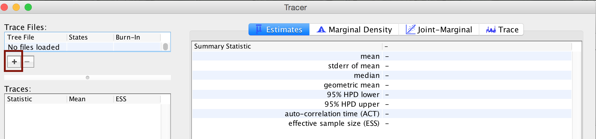 Open Tracer and import the
 bears.log file in the FileImport New Trace File. Or click the button on the left-hand side of the screen to add your log file.
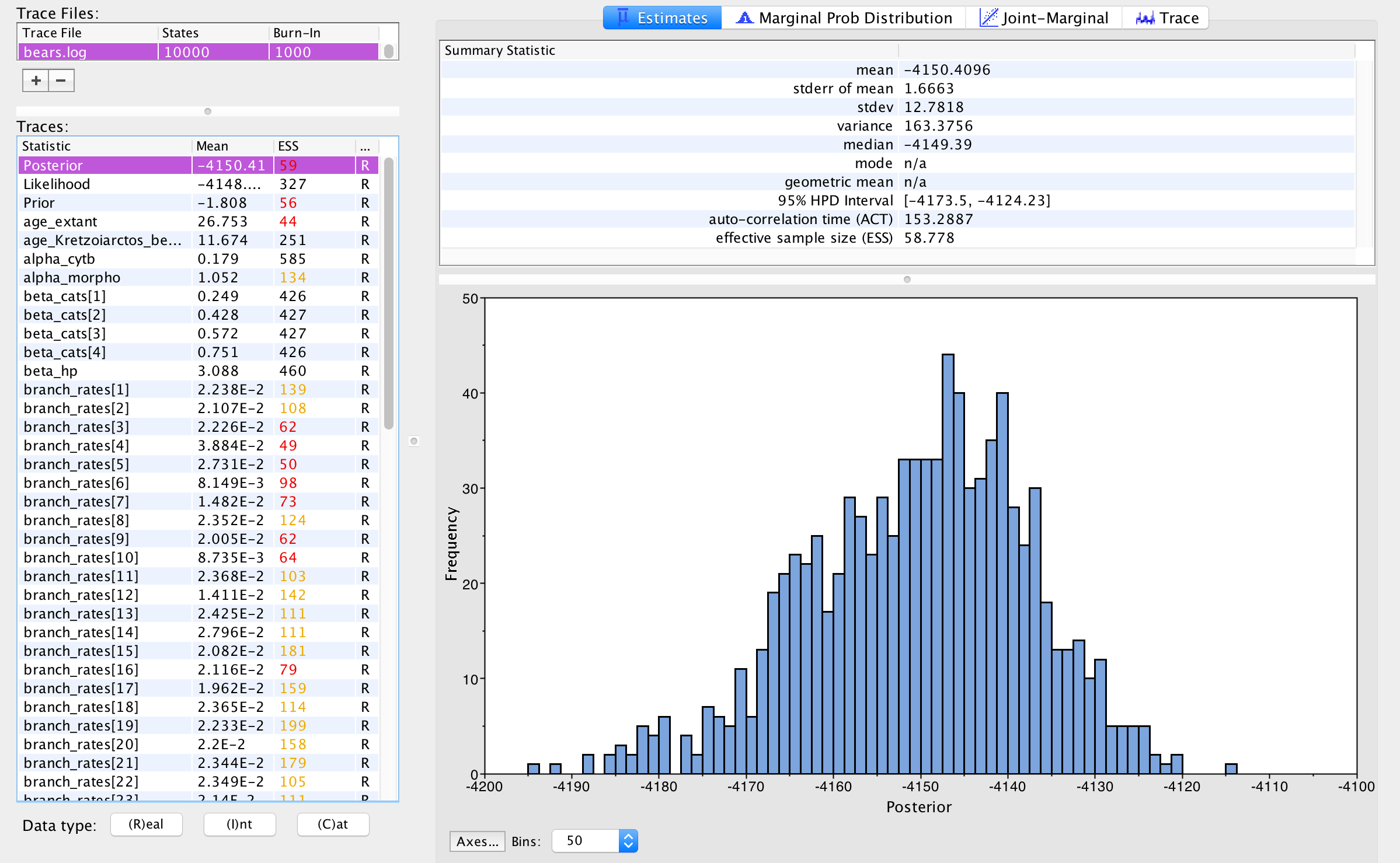 Immediately upon loading your file, you will see the list of Trace Files on the left-hand side (you can load multiple files). The bottom left section, called Traces, provides a list of every parameter in the log file, along with the mean and the effective sample size (ESS) for the posterior sample of that parameter. The ESS statistic provides a measure of the number of independent draws in our sample for a given parameter. This quantity will typically be much smaller than the number of generations of the chain. In Tracer, poor to fair values for the ESS will be colored red and yellow. You will likely see a lot of red and yellow numbers because the MCMC runs in this exercise are too short to effectively sample the posterior distributions of most parameters. A much longer analysis is provided in the
 output directory.
The inspection window for your selected parameter is the Estimates window, which shows a histogram and summary statistics of the values sampled by the Markov chain. Figure 6 shows the marginal distribution of the Posterior statistic for the bears.log file in the output directory.
Look through the various parameters and statistics in the list of Traces.
Are there any parameters that have really low ESS? Why do you think that might be?
Next, we can click over to the Trace window. This window shows us the samples for a given parameter at each iteration of the MCMC. The left side of the chain has a shaded portion that has been excluded as “burn-in”. Samples taken near the beginning of chain are often discarded or “burned” because the MCMC may not immediately begin sampling from the target posterior distribution, particularly if the starting condition of the chain is far from the region of highest posterior density. Figure 7 shows the trace for the extinction rate.
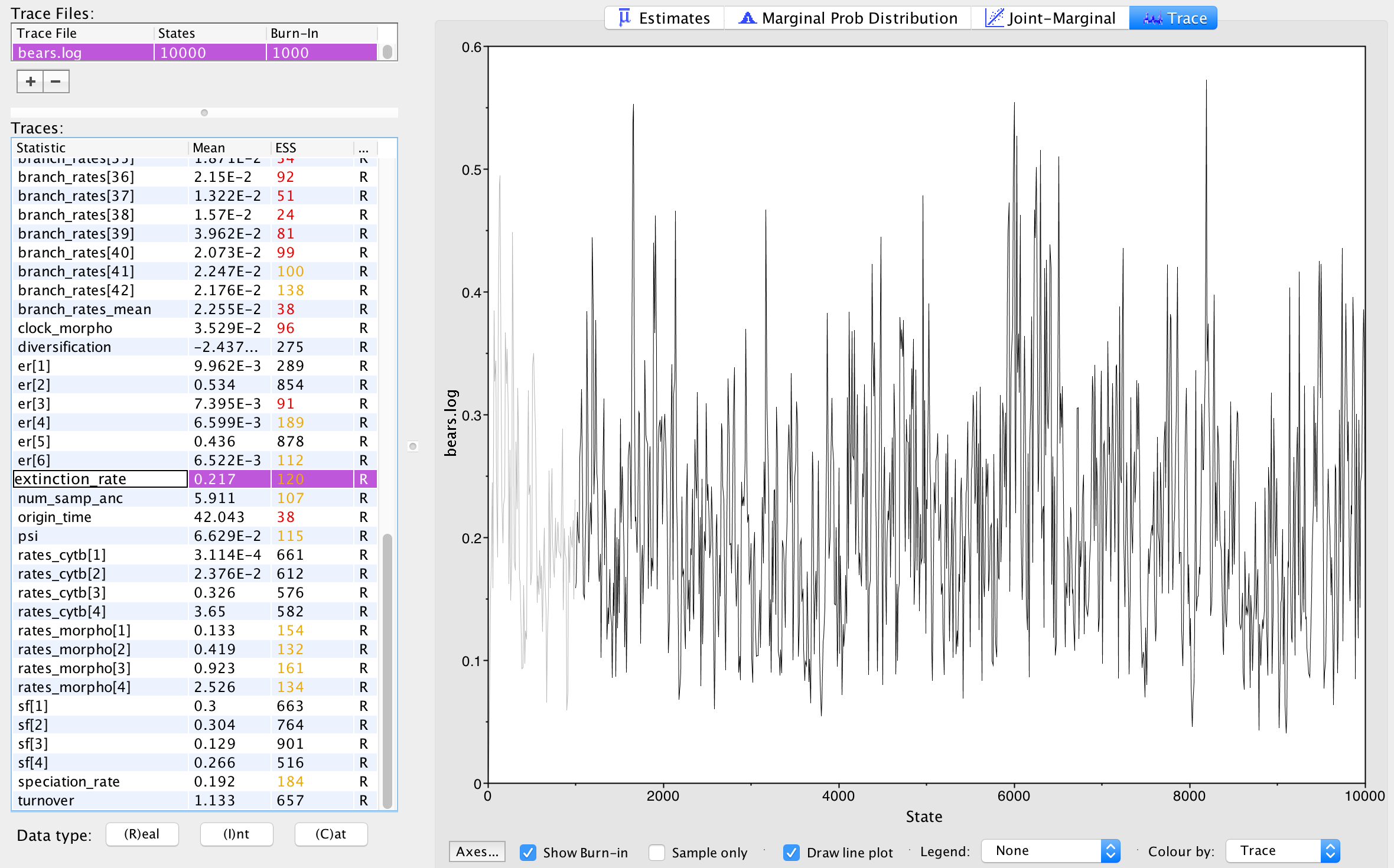 The Trace window allows us to evaluate how well our chain is sampling the target distribution. For a fairly short analysis, the output in figure \[fig:tracer-extinction-trace\] shows reasonable mixing—there is no consistent pattern or trend in the samples, nor are there long intervals where the statistic does not change. The presence of a trend or large leaps in a parameter value might indicate that your MCMC is not mixing well. You can read more about MCMC tuning and improving mixing in the tutorials Intro to MCMC and MCMC Algorithms.
Look through the traces for your parameters.
Are there any parameters in your log files that show trends or large leaps? What steps might you take to solve these issues?
In Tracer you can view the marginal probability distributions of your parameters in the Marginal Prob Distribution window. Using this tool, you can compare the distributions of several different parameters (by selecting them both).
Go to the diversification parameter in the Marginal Prob Distribution window.
What is the mean value estimated for the net diversification rate (\(d\))? What does the marginal distribution tell you about the net diversification? (Hint: \(d = \lambda - \mu\))
While specifying the model, remember that we created several deterministic nodes that represent parameters that we would like to estimate, including the net diversification rate. Tracer allows us to view the summaries of these parameters since they appear in our log files.
Go to the age_extant parameter in the Estimates window.
What is the mean and 95% highest posterior density of the age of the MRCA for all living bears?
Since you have evaluated several of the parameters by viewing the trace files and the ESS values, you may be aware that the MCMC analysis you conducted for this tutorial did not sufficiently sample the joint posterior distribution of phylogenetic parameters. More explicitly, your run has not converged. It is not advisable to base your conclusions on such a run and it will be critical to perform multiple, independent runs for many more MCMC cycles. For further discussion of recommended MCMC practices in RevBayes, please see the Intro to MCMC and MCMC Algorithms tutorials.
Summarize Tree
In addition to evaluating the performance and sampling of an MCMC run using numerical parameters, it is also important to inspect the sampled topology and tree parameters. This is a difficult endeavor, however. One tool for evaluating convergence and mixing of the tree samples is RWTY (Warren et al. 2016). In this tutorial, we will only summarize the sampled trees, but we encourage you to consider approaches for assessing the performance of the MCMC with respect to the tree topology.
Ultimately, we are interested in summarizing the sampled trees and branch times, given that our MCMC has sampled all of the important parameters in proportion to their posterior probabilities. RevBayesincludes some functions for summarizing the tree topology and other tree parameters.
We will complete this part of the tutorial using RevBayesinteractively. Begin by running the RevBayesexecutable. You should do this from within the RB_TotalEvidenceDating_FBD_Tutorial directory.
In Unix systems, type the following in your terminal (if the RevBayesbinary is in your path):
Read in the MCMC sample of trees from file.
trace = readTreeTrace("output/bears.trees")By default, a burn-in of 25% is used when creating the tree trace (250 trees in our case). You can specify a different burn-in fraction, say 50%, by typing the command .
Now we will use the mccTree() function to return a maximum clade credibility (MCC) tree. The MCC tree is the tree with the maximum product of the posterior clade probabilities. When considering trees with sampled ancestors, we refer to the maximum sampled ancestor clade credibility (MSACC) tree (Gavryushkina et al. 2016).
mccTree(trace, file="output/bears.mcc.tre" )When there are sampled ancestors present in the tree, visualizing the tree can be fairly difficult in traditional tree viewers. We will make use of a browser-based tree viewer called IcyTree, created by Tim Vaughan. IcyTree has many unique options for visualizing phylogenetic trees and can produce publication-quality vector image files (i.e.,SVG). Additionally, it correctly represents sampled ancestors on the tree as nodes, each with only one descendant (Fig. 8).
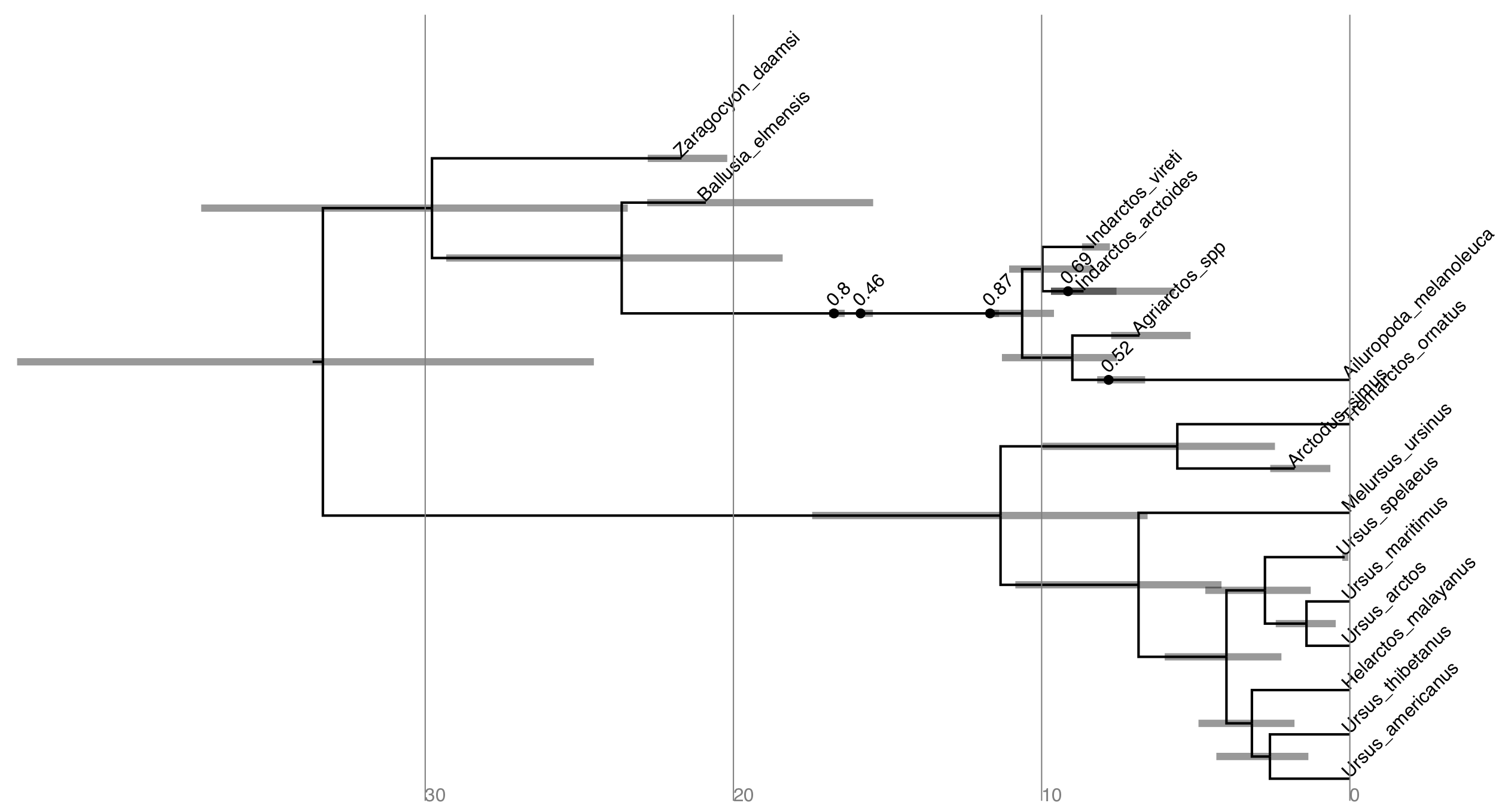
Navigate to http://tgvaughan.github.io/icytree and open the file output/bears.mcc.tre in IcyTree.
Try to replicate the tree in Fig. 8. (Hint: StyleMark Singletons) Why might a node with a sampled ancestor be referred to as a singleton?
How can you see the names of the fossils that are putative sampled ancestors?
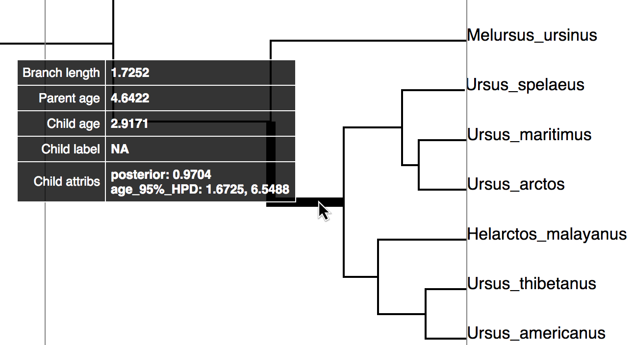
Try mousing over different branches (see Fig. 9). What are the fields telling you? What is the posterior probability that Zaragocyon daamsi is a sampled ancestor?
Another newly available web-based tree viewer is Phylogeny.IO (Jovanovic and Mikheyev 2016). Try this site for a different way to view the tree.
 ## References
Abella, J, P Montoya, and J Morales. 2011. “Una Nueva Especie de Agriarctos (Ailuropodinae, Ursidae, Carnivora) En La Localidad de Nombrevilla 2 (Zaragoza, España).” Estudios Geológicos 67 (2): 187–91.
Abella, Juan, David M. Alba, Josep M. Robles, Alberto Valenciano, Cheyenn Rotgers, Raül Carmona, Plinio Montoya, and Jorge Morales. 2012. “Kretzoiarctos Gen. Nov., the Oldest Member of the Giant Panda Clade.” PLoS One 17: e48985.
Andrews, P, and H Tobien. 1977. “New Miocene Locality in Turkey with Evidence on the Origin of Ramapithecus and Sivapithecus.” Nature 268 (5622): 699.
Baryshnikov, Gennady F. 2002. “Late Miocene Indarctos Punjabiensis Atticus (Carnivora, Ursidae) in Ukraine with Survey of Indarctos Records from the Former USSR.” Russian J. Theriol 1 (2): 83–89.
Bjork, Philip Reese. 1970. “The Carnivora of the Hagerman Local Fauna (Late Pliocene) of Southwestern Idaho.” Transactions of the American Philosophical Society 60 (7): 3–54.
Bouckaert, Remco, Joseph Heled, Denise Kühnert, Tim Vaughan, Chieh-Hsi Wu, Dong Xie, Marc A Suchard, Andrew Rambaut, and Alexei J Drummond. 2014. “BEAST 2: a software platform for Bayesian evolutionary analysis.” PLoS Computational Biology 10 (4). Public Library of Science: e1003537.
Churcher, CS, AV Morgan, and LD Carter. 1993. “Arctodus Simus from the Alaskan Arctic Slope.” Canadian Journal of Earth Sciences 30 (5): 1007–13.
Clark, John, and Thomas Edgar Guensburg. 1972. Arctoid Genetic Characters as Related to the Genus Parictis. Vol. 1150. Chicago, Ill.: Field Museum of Natural History.
Drummond, AJ, SYW Ho, MJ Phillips, and A. Rambaut. 2006. “Relaxed Phylogenetics and Dating with Confidence.” PLoS Biology 4 (5): e88.
Drummond, A.J., M.A. Suchard, D. Xie, and A. Rambaut. 2012. “Bayesian Phylogenetics with Beauti and the Beast 1.7.” Molecular Biology and Evolution 29. SMBE: 1969–73.
Felsenstein, Joseph. 1992. “Phylogenies from Restriction Sites: A Maximum-Likelihood Approach.” Evolution 46 (1). [Society for the Study of Evolution, Wiley]: 159–73. http://www.jstor.org/stable/2409811.
Foote, Michael. 1996. “On the Probability of Ancestors in the Fossil Record.” Paleobiology 22: 141–51.
Gavryushkina, Alexandra, Tracy A. Heath, Daniel T. Ksepka, Tanja Stadler, David Welch, and Alexei J. Drummond. 2016. “Bayesian Total-Evidence Dating Reveals the Recent Crown Radiation of Penguins.” Systematic Biology. https://doi.org/10.1093/sysbio/syw060.
Geraads, Denis, Tanju Kaya, Serdar Mayda, and others. 2005. “Late Miocene Large Mammals from Yulafli, Thrace Region, Turkey, and Their Biogeographic Implications.” Acta Palaeontologica Polonica 50 (3): 523–44.
Ginsburg, Léonard, and Jorge Morales. 1998. “Les Hemicyoninae (Ursidae, Carnivora, Mammalia) et les formes apparentées du Miocène inférieur et moyen d’Europe occidentale.” In Annales de Paléontologie, 84:71–123. 1. Elsevier.
Ginsburg, L, and J Morales. 1995. “Zaragocyon Daamsi N. Gen. Sp. Nov., Ursidae Primitif Du Miocène Inférieur d’Espagne.” Comptes Rendus de L’Académie Des Sciences. Série 2. Sciences de La Terre et Des Planètes 321 (9). Elsevier: 811–15.
Heath, T. A., and B. R. Moore. 2014. “Bayesian Inference of Species Divergence Times.” In Bayesian Phylogenetics: Methods, Algorithms, and Applications, edited by M.-H. Chen, L. Kuo, and P. O. Lewis, 277–318. Chapman & Hall/Crc Mathematical and Computational Biology. Boca Raton, FL: Chapman & Hall/CRC.
Heath, Tracy A, John P Huelsenbeck, and Tanja Stadler. 2014. “The fossilized birth-death process for coherent calibration of divergence-time estimates.” Proceedings of the National Academy of Sciences 111 (29). National Acad Sciences: E2957–E2966.
Heizmann, E, L Ginsburg, and C Bulot. 1980. “Prosansanosmilus Peregrinus, Ein Neuer Machairodontider Felidae Aus Dem Miozän Deutschlands Und Frankreichs.” Stuttgarter Beitr. Naturk. B 58: 1–27.
Höhna, Sebastian, Tracy A. Heath, Bastien Boussau, Michael J. Landis, Fredrik Ronquist, and John P. Huelsenbeck. 2014. “Probabilistic Graphical Model Representation in Phylogenetics.” Systematic Biology 63 (5): 753–71. https://doi.org/10.1093/sysbio/syu039.
Höhna, Sebastian, Michael J. Landis, and Tracy A Heath. 2017. “Phylogenetic Inference Using RevBayes.” Current Protocols in Bioinformatics.
Jin, Changzhu, Russell L Ciochon, Wei Dong, Robert M Hunt, Jinyi Liu, Marc Jaeger, and Qizhi Zhu. 2007. “The First Skull of the Earliest Giant Panda.” Proceedings of the National Academy of Sciences 104 (26): 10932–7.
Jovanovic, Nikola, and Alexander S Mikheyev. 2016. “Interactive Web-Based Visualization of Phylogenetic Trees Using Phylogeny. IO.” PeerJ Preprints 4. PeerJ Inc. San Francisco, USA: e2579v1.
Krause, Johannes, Tina Unger, Aline Noçon, Anna-Sapfo Malaspinas, Sergios-Orestis Kolokotronis, Mathias Stiller, Leopoldo Soibelzon, et al. 2008. “Mitochondrial Genomes Reveal an Explosive Radiation of Extinct and Extant Bears Near the Miocene-Pliocene Boundary.” BMC Evolutionary Biology 8 (1). BioMed Central Ltd: 220.
Lewis, Paul O. 2001. “A Likelihood Approach to Estimating Phylogeny from Discrete Morphological Character Data.” Systematic Biology 50 (6). Oxford University Press: 913–25.
Loreille, Odile, Ludovic Orlando, Marylène Patou-Mathis, Michel Philippe, Pierre Taberlet, and Catherine Hänni. 2001. “Ancient DNA Analysis Reveals Divergence of the Cave Bear, Ursus Spelaeus, and Brown Bear, Ursus Arctos, Lineages.” Current Biology 11 (3): 200–203.
Montoya, P, L Alcalá, and J Morales. 2001. “Indarctos (Ursidae, Mammalia) from the Spanish Turolian (Upper Miocene).” Scripta Geologica 122: 123–51.
Rambaut, Andrew, and Alexei J. Drummond. 2011. “Tracer V1.5.” http://tree.bio.ed.ac.uk/software/tracer/.
Ronquist, F., and J.P. Huelsenbeck. 2003. “MrBayes 3: Bayesian phylogenetic inference under mixed models.” Bioinformatics 19 (12). Oxford Univ Press: 1572–4.
Ronquist, Fredrik, Seraina Klopfstein, Lars Vilhelmsen, Susanne Schulmeister, Debra L Murray, and Alexandr P Rasnitsyn. 2012. “A Total-Evidence Approach to Dating with Fossils, Applied to the Early Radiation of the Hymenoptera.” Systematic Biology 61 (6). Oxford University Press: 973–99.
Stadler, T. 2010. “Sampling-through-time in birth-death trees.” Journal of Theoretical Biology 267 (3). Elsevier: 396–404.
Stadler, Tanja, Alexandra Gavryushkina, Rachel Warnock, Alexei J Drummond, and Tracy A Heath. 2017. “The Fossilized Birth-Death Model for the Analysis of Stratigraphic Range Data Under Different Speciation Concepts.” arXiv Preprint arXiv:1706.10106.
Thorne, Jeffrey L, and Hirohisa Kishino. 2002. “Divergence Time and Evolutionary Rate Estimation with Multilocus Data.” Systematic Biology 51 (5). Oxford University Press: 689–702.
Warren, DL, A Geneva, DL Swofford, and R Lanfear. 2016. “Rwty: R We There yet.” A Package for Visualizing MCMC Convergence in Phylogenetics.
Zhang, Chi, Tanja Stadler, Seraina Klopfstein, Tracy A. Heath, and Fredrik Ronquist. 2016. “Total-Evidence Dating Under the Fossilized Birth-Death Process.” Systematic Biology 65 (2): 228–49. https://doi.org/10.1093/sysbio/syv080.
Zuckerkandl, E., and L. Pauling. 1962. “Molecular Disease, Evolution, and Genetic Heterogeneity.” In Horizons in Biochemistry, edited by M. Kasha and B. Pullman, 189–225. Academic Press, New York.